ABYSS_16S
Diversity and biogeography of bathyal and abyssal seafloor Bacteria and Archaea along a Mediterranean – Atlantic gradient ================
- PART 1: Preparation of DADA2 output for further statistical analysis
- PART 2: Statistical analysis and production of
figures
- Figure 1: Map of samples and PCA
- Figure 2: Overall distance-decay relationship and variation partitioning
- Figure 3: Evolution of the distance-decay with horizon depth
- Figure 4: Ordinations (nMDS) and permanova
- Figure 5: Local-scale analysis: DDR, correlation with environment, variation partitioning and biomarkers of horizon vs site
- Supplementary figures and analysis
This is a reproducible workflow for the 16S metabarcoding analysis of the paper “Biodiversity and biogeography of benthic bacteria and archaea across the Mediterranean - Atlantic transition”.
PART 1: Preparation of DADA2 output for further statistical analysis
The first part of this script aims at generating all the files needed for further analysis. It will thus:
- input the raw ASV and taxonomy tables obtained from DADA2 (with assignation using RDP on the Silva 138 database with a bootstrap of 80)
- merge samples that were duplicated during sequencing
- implement the decontam package to remove contaminants
- create a normalized phyloseq object using package metagenomeSeq
library(here)
library(data.table)
library(vegan)
library(phyloseq)
library(ggplot2)
library(decontam)

here()
## [1] "/scratch/work/blandine/02_Med_Atl/16S_fuhrman/ABYSS_16S"
theme_1 <- theme(axis.title.x = element_text(face="bold",size=16),
                 axis.text.x = element_text(angle=0, colour = "black", vjust=1, hjust = 1, size=14),
                 axis.text.y = element_text(colour = "black", size=14),
                 axis.title.y = element_text(face="bold",size=16),
                 plot.title = element_text(size = 18),
                 legend.title =element_text(size = 14),
                 legend.text = element_text(size = 14),
                 legend.position="right",
                 legend.key.size = unit(0.50, "cm"),
                 strip.text.x = element_text(size=12, face="bold"),
                 strip.text.y = element_text(size=12, face="bold"),
                 panel.background = element_blank(),
                 panel.border = element_rect(fill = NA, colour = "black"),
                 strip.background = element_rect(colour="black"))
scale_horizon <- c("cyan", "gold", "chartreuse", "royalblue", "purple", "red", "orange")

scale_geo_zone = c("Atlantic_Ocean" = "darkblue", "Transition" = "gold", "Mediterranean_Sea" = "darkgreen")

scale_location = c("North Atlantic 4000-5000m" = "darkblue", "Azores 1200-1500m (Formigas seamount)" = "dodgerblue",
                     "SW Portugal 1920m (Ormonde seamount)" = "red", "Gulf of Cádiz 470m (Gazul mud volc.)" = "darkorange",
                     "Alborán Sea 300-800m (SdO gullot)" = "gold", "West Med 2000-3000m" = "seagreen",
                     "NW Med 334m" = "yellowgreen", "East Med 3000-3500m" = "darkgreen")

scale_taxon = c("#FF4500", "grey26", "#32CD32", "#4169e1", "#e0e0e0", "#00bfff", "#99ff99", "#a020f0", "#006400", "#00FFFF",
                "#FFD700", "#FF1493", "#DAA520", "#8B4513", "#FFA500", "#6B8E23", "darkblue", "mediumorchid3", "#508578")

 scale_55 = c("grey26", "royalblue", "chartreuse3",  "red", "darkorange","cyan2", "darkgreen", "deepskyblue", "mediumorchid3","#89C5DA", "#DA5724", "#74D944", "#C84248", "#673770", "#D3D93E", "#38333E", "#508578", "#D7C1B1", "#689030",   "#AD6F3B", "#CD9BCD", "#D14285", "#6DDE88", "#652926", "#7FDCC0", "#8569D5", "#5E738F", "#D1A33D", "#8A7C64", "#599861", "blue4", "yellow1", "violetred", "#990000", "#99CC00", "#003300", "#00CCCC", "#9966CC", "#993366", "#990033", "#4863A0", "#000033", "#330000", "#00CC99", "#00FF33", "#00CCFF", "#FF9933", "#660066", "#FF0066", "#330000", "#CCCCFF", "#3399FF", "#66FFFF", "#B5EAAA","#FFE87C")
1- Input raw data
ASVs <- read.table(here("docs/10_ASVs_counts.tsv"), sep = "\t", header = T, row.names = 1, check.names=FALSE)
TAXO <- read.table(here("docs/10_ASVs_taxonomy.tsv"), sep = "\t", header = T, row.names = 1)
# the names of the ASVs are Cluster_1 to Cluster_265926, the corresponding sequences can be found in 10_ASVs.fasta

ASVs <- otu_table(ASVs, taxa_are_rows = TRUE)
TAXO <- tax_table(as.matrix(TAXO))
colnames(TAXO) <- c("Kingdom", "Phylum", "Class", "Order", "Family", "Genus", "Species",
                    "boot.Kingdom", "boot.Phylum", "boot.Class", "boot.Order", "boot.Family", "boot.Genus", "boot.Species")

ps_sed <- phyloseq(ASVs, TAXO)
rm(ASVs, TAXO)
To start with we have 265,926 taxa and 415 samples.
2- Merge duplicated samples
In some of the sequencing runs, libraries were deposited on 2 lanes of Hiseq 2500 machines, so the sequence files are duplicated. There are 161 duplicated samples. Let’s first check if the difference is great between duplicate samples.
duplicated_samples <- data.frame("Sample_ID" = sample_names(ps_sed), "Sequencing" = 0)
duplicated_samples$Sequencing[grepl("_A$", duplicated_samples$Sample_ID)] <- "Lane1"
duplicated_samples$Sequencing[grepl("_B$", duplicated_samples$Sample_ID)] <- "Lane2"
duplicated_samples$Sequencing[duplicated_samples$Sequencing == 0] <- "Single lane"

sum(duplicated_samples$Sequencing=="Lane1")
## [1] 161
sum(duplicated_samples$Sequencing=="Lane2")
## [1] 161
sum(duplicated_samples$Sequencing=="Single lane")
## [1] 93
# add the info about sequencing to the phyloseq object as sample data for further processing
rownames(duplicated_samples) <- duplicated_samples$Sample_ID
ps_sed <- phyloseq(otu_table(ps_sed), tax_table(ps_sed), sample_data(duplicated_samples))
test <- subset_samples(ps_sed, Sequencing != "Single lane")
test <- prune_taxa(taxa_sums(test)>0, test)

library(metagenomeSeq)
ASV_MR <- phyloseq_to_metagenomeSeq(test)
ASV_MR_nor <- cumNorm(ASV_MR)
ASV_df_nor <- MRcounts(ASV_MR_nor, norm = T)
test_norm <- phyloseq(otu_table(ASV_df_nor, taxa_are_rows = TRUE), tax_table(test), sample_data(test))
test_norm <- prune_taxa(taxa_sums(test_norm)>0, test_norm)

rm(ASV_MR, ASV_MR_nor, ASV_df_nor)

NMDS.test.ord <- ordinate(test_norm, "NMDS", "bray")

sampleplot <-  plot_ordination(test_norm, NMDS.test.ord, type = "samples", color = "Sequencing")
sampleplot + theme_1
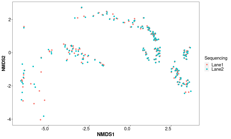
Duplicated samples are more similar together than with other samples. Since this is the case, the duplicated samples will be merged, and counts summed by phyloseq since it will not affect downstream analysis (work on either the normalized or relative abundance dataset).
# Let's remove the identifier of duplicated samples from SampleID, this factor will then be used to merge
ps_sed@sam_data$Sample_ID <- sub("_A$|_B$", "", ps_sed@sam_data$Sample_ID)
ps_sed <- merge_samples(ps_sed, "Sample_ID", fun = sum)
ps_sed@sam_data <- NULL

# the sample number is now ok, we can add the proper metadata table. This table can be found in the supplementary data of the paper.
metadata <- read.table(here("docs/Table_S1_metadata.csv"), sep = ";", header = T, row.names = 1)
# three samples were not sequenced, and the status column is not useful here
metadata <- metadata[!(metadata$Status == "Sequencing failed"),]
metadata$Status <- NULL
META <- sample_data(metadata)

ps_sed <- phyloseq(t(otu_table(ps_sed)), tax_table(ps_sed), META)
We are now left with 254 samples and still 265,926 taxa.
3- Remove unwanted taxa and contaminants
Let’s remove sequences assigned to Eukaryota, Chloroplast and Mitochondria.
# remove Eukaryota
levels(as.factor(ps_sed@tax_table[,1]))
## [1] "Archaea" "Bacteria" "Eukaryota"
ps_sed_refined <- subset_taxa(ps_sed, Kingdom != "Eukaryota")

sum(is.na(ps_sed_refined@tax_table[,1]))
## [1] 0
# check for unwanted like chloroplast or mitochondria
# be subset_taxa removes any NA as well if not careful!
ps_sed_refined <- subset_taxa(ps_sed_refined, (Order!="Chloroplast") | is.na(Order))
ps_sed_refined <- subset_taxa(ps_sed_refined, (Family!="Mitochondria") | is.na(Family))
We now have 262,614 taxa left.
# we will track the number of reads in each sample throught the processing of the dataset
df_read_track <- data.table(Sample_ID=sample_names(ps_sed), Raw_sequence_number=sample_sums(ps_sed),
                            Refined_taxonomy=sample_sums(ps_sed_refined))
rownames(df_read_track) <- sample_names(ps_sed)
How many ASVs in the controls?
ps_control <- subset_samples(ps_sed_refined, Type == "control")
ps_control <- prune_taxa(taxa_sums(ps_control)>0, ps_control)

cat("Percentage of reads that are found in negative controls = ",
    signif((sum(sample_sums(ps_control))/sum(sample_sums(ps_sed@otu_table))*100),4))
## Percentage of reads that are found in negative controls = 9.785
1951 taxa present in control samples, that represent almost 10% of the total number of reads. Let’s use decontam to try and remove contaminants from the dataset.
sample_data(ps_sed_refined)$is.neg <- sample_data(ps_sed_refined)$Type == "control"
contamdf.prev05 <- isContaminant(ps_sed_refined, method="prevalence", neg="is.neg", threshold=0.5)
table(contamdf.prev05$contaminant)
##
##  FALSE   TRUE
## 262152    462
# Make phyloseq object of presence-absence in negative controls and true samples
ps.pa <- transform_sample_counts(ps_sed_refined, function(abund) 1*(abund>0))
ps.pa.neg <- prune_samples(sample_data(ps.pa)$Type == "control", ps.pa)
ps.pa.pos <- prune_samples(sample_data(ps.pa)$Type == "sample", ps.pa)

# Make data.frame of prevalence in positive and negative samples
df.pa <- data.frame(pa.pos=taxa_sums(ps.pa.pos), pa.neg=taxa_sums(ps.pa.neg),
                      contaminant=contamdf.prev05$contaminant)
ggplot(data=df.pa, aes(x=pa.neg, y=pa.pos, color=contaminant)) + geom_point() +
  xlab("Prevalence (Negative Controls)") + ylab("Prevalence (True Samples)")
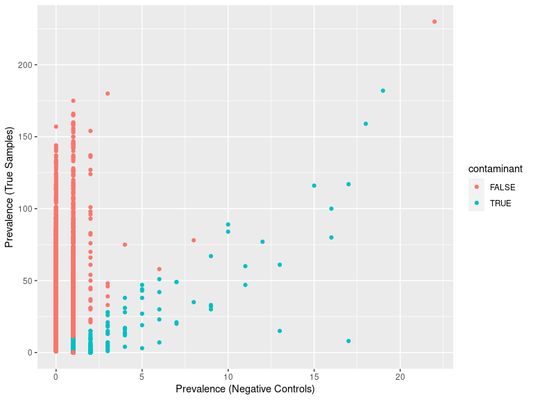
ps_sed_decontam <- prune_taxa(rownames(contamdf.prev05)[contamdf.prev05$contaminant == FALSE], ps_sed_refined)
decontam_controls <- subset_samples(ps_sed_decontam, Type == "control")
decontam_controls <- prune_taxa(taxa_sums(decontam_controls)>0, decontam_controls)

cat("Percentage of reads that are found in negative controls = ", signif((sum(sample_sums(decontam_controls))/sum(sample_sums(ps_sed_decontam@otu_table))*100),4))
## Percentage of reads that are found in negative controls = 9.573
p <- plot_bar(decontam_controls, fill = "Phylum") +
  scale_fill_manual(values = scale_55) +
  scale_colour_manual(values = scale_55)
p
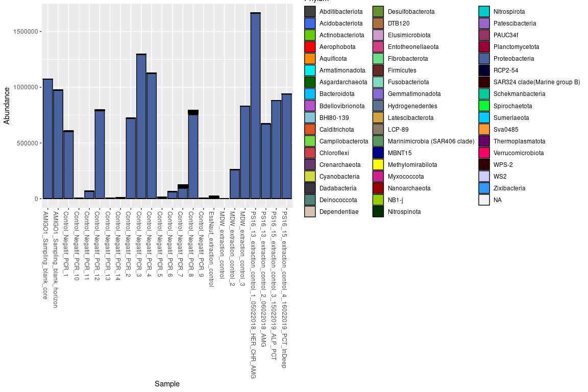
After decontam, the 1489 ASVs still present in control samples still
represent around 9.5% of the total number of reads.
1 ASV in particular makes up for 99% of the reads in control samples.
This is due to a contamination in the Taq-Phusion used.
This ASV is mostly found in samples with low DNA content after
extraction, it will be completely removed from the dataset.
# list ASVs by importance in the controls + add % they represent
total_reads <- sum(taxa_sums(decontam_controls))
ASVpercent <-  data.frame(percent = sort((taxa_sums(decontam_controls) / total_reads * 100), decreasing = TRUE))

ps_sed_decontam <- subset_taxa(ps_sed_decontam, taxa_names(ps_sed_decontam) != rownames(ASVpercent)[1])
# should be 262,151 taxa
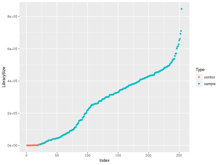
Checking the library sizes (controls should be on the bottom left)
df <- as.data.frame(sample_data(ps_sed_decontam)) # Put sample_data into a ggplot-friendly data.frame
df$LibrarySize <- sample_sums(ps_sed_decontam)
df <- df[order(df$LibrarySize),]
df$Index <- seq(nrow(df))
ggplot(data=df, aes(x=Index, y=LibrarySize, color=Type)) + geom_point()
Tracking the reads by samples through preprocessing
df_decontam <- data.frame(Sample_ID=sample_names(ps_sed_decontam),
                          After_decontam=sample_sums(ps_sed_decontam))
# after decontam but before removing controls
df_read_track <- merge(df_read_track, df_decontam, by = "Sample_ID", all.x = TRUE, all.y = TRUE)
df_read_track$Percent_retained <- df_read_track$After_decontam  * 100 / df_read_track$Raw_sequence_number
Removing controls from the dataset
ps_sed_decontam <- subset_samples(ps_sed_decontam, Type == "sample")
# number of samples: 230
Let’s check the number of reads by library to remove the ones that are too low after decontamination
readsumsdf = data.frame(nreads = sort(sample_sums(ps_sed_decontam), TRUE), sorted = 1:nsamples(ps_sed_decontam), type = "Samples")

p = ggplot(readsumsdf, aes(x = sorted, y = nreads)) + geom_bar(stat = "identity", position = "stack", fill="gray", width = 0.8)
p + ggtitle("Total number of reads by sample for full dataset")
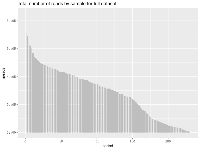
max(sort(sample_sums(ps_sed_decontam), decreasing = TRUE))
## [1] 847227
mean(sort(sample_sums(ps_sed_decontam), decreasing = TRUE))
## [1] 292456.7
min(sort(sample_sums(ps_sed_decontam), decreasing = TRUE))
## [1] 3834
The chosen threshold is 40,000 reads by sample (to keep as many samples as possible without lowering the number too much)
# Samples to be removed:
sample_names(subset_samples(ps_sed_decontam, sample_sums(ps_sed_decontam) < 40000))
##  [1] "AMIGO1_Site0_CT2_0-1"   "AMIGO1_Site1_CT1_3-5"   "AMIGO1_Site1_CT3_5-10"
##  [4] "AMIGO1_Site1_CT4_3-5"   "AMIGO1_Site2_CT1_3-5"   "AMIGO1_Site2_CT1_5-10"
##  [7] "AMIGO1_Site3_CT1_0-1"   "AMIGO1_Site3_CT1_1-3"   "AMIGO1_Site3_CT1_3-5"
## [10] "AMIGO1_Site3_CT1_5-10"  "AMIGO1_Site3_CT2_10-15" "AMIGO1_Site3_CT2_5-10"
## [13] "AMIGO1_Site3_CT3_0-1"   "AMIGO1_Site3_CT3_1-3"   "AMIGO1_Site3_CT3_3-5"
## [16] "CANHROV_Site1_CT1_5-10" "CANHROV_Site1_CT2_5-10" "MDW_ST68_CT1_15-30"
## [19] "PCT_I_CT4_5-10"         "PCT_T_CT1_10-15"
ps_sed_decontam <-  prune_samples(sample_sums(ps_sed_decontam) >= 40000, ps_sed_decontam)
ps_sed_decontam <- prune_taxa(taxa_sums(ps_sed_decontam)>0, ps_sed_decontam)
ps_sed_decontam
## phyloseq-class experiment-level object
## otu_table()   OTU Table:         [ 260567 taxa and 210 samples ]
## sample_data() Sample Data:       [ 210 samples by 28 sample variables ]
## tax_table()   Taxonomy Table:    [ 260567 taxa by 14 taxonomic ranks ]
# 210 samples left (20 removed), 260,567 taxa left

ps_sed_decontam@sam_data$is.neg = NULL
ps_sed <- ps_sed_decontam
In the full dataset, there are 210 samples and 260,567 taxa.
# Aggregate horizons under 30 cm
ps_sed@sam_data$Horizon <- sub("30_40|30_50|30_45|40_50", "30+", ps_sed@sam_data$Horizon)
ps_sed@sam_data$Horizon <- factor(ps_sed@sam_data$Horizon, levels = c("0_1", "1_3", "3_5", "5_10", "10_15", "15_30", "30+"))

# location with depth for map, PCA, NMDS
ps_sed@sam_data$Location_depth <- paste(ps_sed@sam_data$Location, ps_sed@sam_data$Depth_range)
ps_sed@sam_data$Location_depth <- gsub("Alboran Sea \\(SdO gullot) 0 - 1000m", "Alborán Sea 300-800m \\(SdO gullot)", ps_sed@sam_data$Location_depth)
ps_sed@sam_data$Location_depth <- gsub("Azores \\(Formigas seamount) 1000 - 2000m", "Azores 1200-1500m \\(Formigas seamount)",
                                       ps_sed@sam_data$Location_depth)
ps_sed@sam_data$Location_depth <- gsub("Gulf of Cadiz \\(Gazul mud volcano) 0 - 1000m", "Gulf of Cádiz 470m \\(Gazul mud volc.)",
                                       ps_sed@sam_data$Location_depth)
ps_sed@sam_data$Location_depth <- gsub("Southwest Portugal \\(Ormonde seamount) 1000 - 2000m", "SW Portugal 1920m \\(Ormonde seamount)",
                                       ps_sed@sam_data$Location_depth)
ps_sed@sam_data$Location_depth <- gsub("Mediterranean \\(abyssal plain) 3000 - 4000m", "East Med 3000-3500m", ps_sed@sam_data$Location_depth)
ps_sed@sam_data$Location_depth <- gsub("North Atlantic \\(abyssal plain) 4000 - 5000m", "North Atlantic 4000-5000m", ps_sed@sam_data$Location_depth)
ps_sed@sam_data$Location_depth <- gsub("Mediterranean \\(undersea canyon) 2000 - 3000m", "West Med 2000-3000m", ps_sed@sam_data$Location_depth)
ps_sed@sam_data$Location_depth <- gsub("Mediterranean \\(passive margin) 2000 - 3000m", "West Med 2000-3000m", ps_sed@sam_data$Location_depth)
ps_sed@sam_data$Location_depth <- gsub("Mediterranean \\(passive margin) 0 - 1000m", "NW Med 334m", ps_sed@sam_data$Location_depth)
ps_sed@sam_data$Location_depth <- gsub("Mediterranean \\(abyssal plain) 2000 - 3000m", "West Med 2000-3000m", ps_sed@sam_data$Location_depth)
levels(as.factor(ps_sed@sam_data$Location_depth))
## [1] "Alborán Sea 300-800m (SdO gullot)"
## [2] "Azores 1200-1500m (Formigas seamount)"
## [3] "East Med 3000-3500m"
## [4] "Gulf of Cádiz 470m (Gazul mud volc.)"
## [5] "North Atlantic 4000-5000m"
## [6] "NW Med 334m"
## [7] "SW Portugal 1920m (Ormonde seamount)"
## [8] "West Med 2000-3000m"
4- Normalize the phyloseq object using metagenomeSeq
library(metagenomeSeq)
# new metadata added
ASV_MR <- phyloseq_to_metagenomeSeq(ps_sed)
ASV_MR <- cumNorm(ASV_MR)
ASV_df_nor <- MRcounts(ASV_MR, norm = T)
ps_sed_norm <- phyloseq(otu_table(ASV_df_nor, taxa_are_rows = TRUE), tax_table(ps_sed), sample_data(ps_sed))
ps_sed_norm <- prune_taxa(taxa_sums(ps_sed_norm)>0, ps_sed_norm)

rm(ASV_df_nor, ASV_MR)
Let’s save the info necessary for the read track table. Optionally, the phyloseq objects can be saved as well.
write.csv(df_read_track, here("docs/track_reads_data_prep.csv"))

saveRDS(ps_sed, here("docs/Ps_MedAtl_decontam_boot80_Silva138.rds"))
saveRDS(ps_sed_norm, here("docs/Ps_MedAtl_decontam_norm_boot80_Silva138.rds"))
PART 2: Statistical analysis and production of figures
The second part of this script will go through the analysis necessary to produce the figures found in the paper.
library(ggthemes)
library(reshape2)
library(RColorBrewer)
library(DESeq2)
library(dplyr)
library(UpSetR)
library(tidyr)
library(stats)
library(geosphere)
library(ggpmisc)
library(broom)
library(simba)
library(patchwork)
library(speedyseq)
library(gridExtra)
library(grid)
library(enmSdm)

here::here()
## [1] "/scratch/work/blandine/02_Med_Atl/16S_fuhrman/ABYSS_16S"
Personnal functions that will be used in the script:
# getting upper triangle matrix from distance suqare matrix
get_upper_tri <- function(matrix){
  matrix[lower.tri(matrix)]<- NA
  return(matrix)
}

# function for easy and faster taxonomy plotting
source(here::here("docs/Function_normalize_counts_by_sample.R"))

# function to make graph for Upset package
graph_for_upset <- function(phylo, parameter){
  data.mat.raref <- psmelt(phylo)
  data.mat.raref <- data.mat.raref[data.mat.raref$Abundance>0,]

  data.mat.raref$OTU=factor(data.mat.raref$OTU) # OTUid
  groups <- unique(data.mat.raref[[parameter]])

  graph<-lapply(groups,function(X){
    p <- data.mat.raref[data.mat.raref[[parameter]]==X,]
    unique(p$OTU)
    })
  names(graph)<-groups
  return(graph)
}

# for biomarker analysis
gm_mean = function(x, na.rm=TRUE){
  exp(sum(log(x[x > 0]), na.rm=na.rm) / length(x))
}
Defining orders for factors in our phyloseq objects
# horizon from top to bottom
Horizon_order <- c("0_1", "1_3", "3_5", "5_10", "10_15", "15_30", "30+")

# horizon from deep to top
flipped_horizon <- c("30+", "15_30", "10_15", "5_10", "3_5", "1_3", "0_1")

# location west to east (possibly not useful anymore)
Location_order <- c("North Atlantic (abyssal plain)", "Azores (Formigas seamount)",
                    "Southwest Portugal (Ormonde seamount)", "Gulf of Cadiz (Gazul mud volcano)", "Alboran Sea (SdO gullot)",
                    "Mediterranean (undersea canyon)", "Mediterranean (passive margin)", "Mediterranean (abyssal plain)")

# ordering depth zones from shallow to deep
Depth_zone_order <- c("Upper bathyal (300-800m)", "Lower bathyal (1200-3500m)", "Abyssal (4000m+)")

# geographical zones from West to East
Geo_zone_order <- c("Atlantic_Ocean", "Transition", "Mediterranean_Sea")

# location depth order for map, NMDS, PCA
Loc_depth_order <- c("North Atlantic 4000-5000m", "Azores 1200-1500m (Formigas seamount)", "SW Portugal 1920m (Ormonde seamount)",
                     "Gulf of Cádiz 470m (Gazul mud volc.)", "Alborán Sea 300-800m (SdO gullot)", "West Med 2000-3000m", "NW Med 334m",
                     "East Med 3000-3500m")

# Group orders (DDR)
Group_order <- c("Atlantic Ocean", "Transition", "Mediterranean Sea", "Atlantic - Mediterranean",
                 "Atlantic - Transition", "Mediterranean - Transition")
# Ordering ps_sed_norm
# Location
ps_sed_norm@sam_data$Location <- factor(ps_sed_norm@sam_data$Location, levels = Location_order)
# Horizon
ps_sed_norm@sam_data$Horizon <- factor(ps_sed_norm@sam_data$Horizon, levels = Horizon_order)
# Geographic zone west to east
ps_sed_norm@sam_data$Geo_zone <- factor(ps_sed_norm@sam_data$Geo_zone, levels = Geo_zone_order)
# Location_depth
ps_sed_norm@sam_data$Location_depth <- factor(ps_sed_norm@sam_data$Location_depth, levels = Loc_depth_order)
# Depth zone
ps_sed_norm@sam_data$Zone <- factor(ps_sed_norm@sam_data$Zone, levels = Depth_zone_order)

# Ordering ps_sed
# Location
ps_sed@sam_data$Location <- factor(ps_sed@sam_data$Location, levels = Location_order)
# Horizon
ps_sed@sam_data$Horizon <- factor(ps_sed@sam_data$Horizon, levels = Horizon_order)
# Geographic zone west to east
ps_sed@sam_data$Geo_zone <- factor(ps_sed@sam_data$Geo_zone, levels = Geo_zone_order)
# Location_depth
ps_sed@sam_data$Location_depth <- factor(ps_sed@sam_data$Location_depth, levels = Loc_depth_order)
# Depth zone
ps_sed@sam_data$Zone <- factor(ps_sed@sam_data$Zone, levels = Depth_zone_order)
Creating the phyloseq object with appropriate taxonomy for plotting
# singletons considered are taxa that appear less than 3 times in the whole dataset, remove them
ps_sed_rel <- prune_taxa(taxa_sums(ps_sed) > 2, ps_sed)
ps_sed_rel <- transform_sample_counts(ps_sed_rel, function(x) (x/sum(x)))
# 239,314 taxa

taxo <- data.frame(ps_sed_rel@tax_table)
taxo$Phylum_keep <- taxo$Phylum
taxo <- as.data.table(taxo)

# more resolution in Proteobacteria and Crenarchaeota for clarity
taxo[Class=="Alphaproteobacteria", Phylum:="Proteobac.: Alphaproteobacteria"]
taxo[Class=="Gammaproteobacteria", Phylum:="Proteobac.: Gammaproteobacteria"]
taxo[Class=="Zetaproteobacteria", Phylum:="Proteobac.: Zetaproteobacteria"]
taxo[Class=="Magnetococcia", Phylum:="Proteobac.: Magnetococcia"]
taxo[Phylum=="Proteobacteria" & is.na(Class), Phylum:="Unassigned Proteobacteria"]
taxo[Class=="Bathyarchaeia", Phylum:="Crenarchaeota: Bathyarchaeia"]
taxo[Class=="Nitrososphaeria", Phylum:="Crenarchaeota: Nitrososphaeria"]
taxo[Phylum=="Crenarchaeota", Phylum:="Crenarchaeota (NA)"]

taxo <- as.matrix(taxo)
rownames(taxo) <- taxa_names(ps_sed_rel)

ps_sed_rel <- phyloseq(otu_table(ps_sed_rel), tax_table(taxo), sample_data(ps_sed_rel))

general_taxo_phy <- tax_glom(ps_sed_rel, taxrank=rank_names(ps_sed_rel)[2], NArm=FALSE)

df_phy <- data.frame(general_taxo_phy@tax_table[,c(1:2)])
df_phy$percent <- signif((taxa_sums(general_taxo_phy) * 100 / 210), 3)
df_phy <- df_phy[order(-df_phy$percent),]

# # on garde les 17 premiers
phylum_to_keep <- df_phy$Phylum[1:19]

# # keep chosen phyla and group the rest in "Others"
taxo <- as.data.table(taxo)
taxo$Phylum[(taxo$Phylum %in% phylum_to_keep) == FALSE] <- "Others"

taxo <- as.matrix(taxo)
rownames(taxo) <- taxa_names(ps_sed_rel)

ps_sed_rel <- phyloseq(otu_table(ps_sed_rel), tax_table(taxo), sample_data(ps_sed_rel))

saveRDS(ps_sed_rel, here::here("docs/ps_sed_rel.rds"))
ps_sed_rel <- readRDS(here::here("docs/ps_sed_rel.rds"))
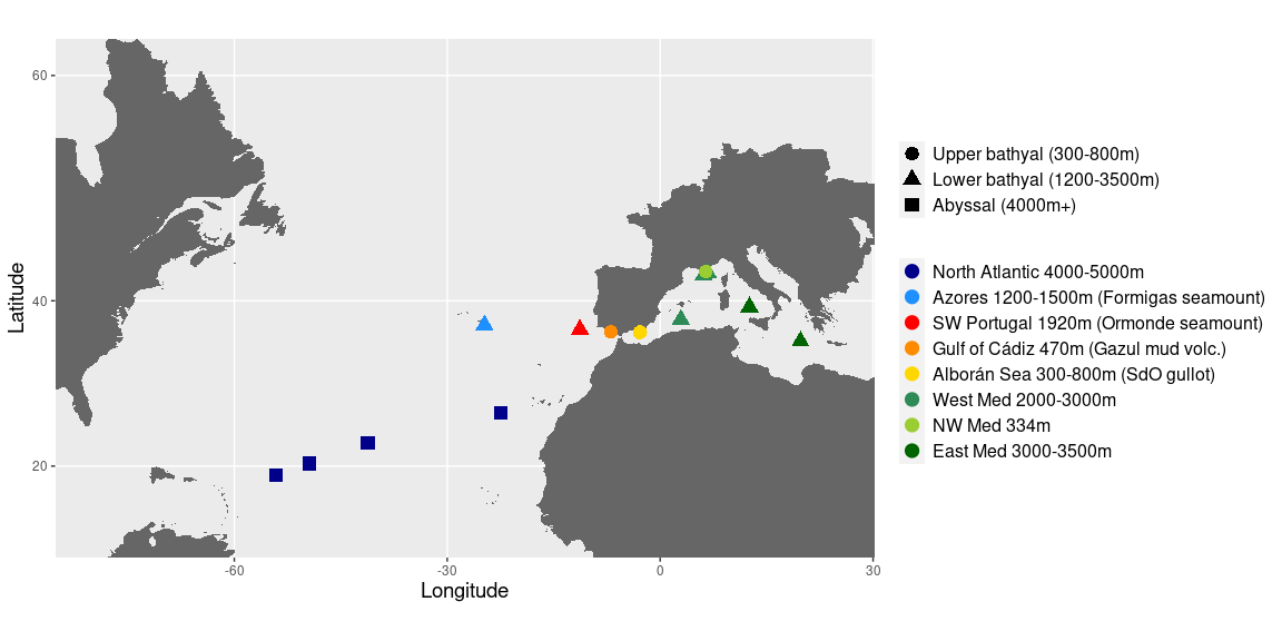
Figure 1: Map of samples and PCA
library(ggmap)
library(maps)

# import data points
coords <- as.data.frame(as.matrix(ps_sed@sam_data))
coords$Longitude <- as.numeric(as.character(coords$Longitude))
coords$Latitude <- as.numeric(as.character(coords$Latitude))

# create column for colors
coords$Colour_map <- coords$Location_depth
coords$Colour_map <- factor(coords$Colour_map, levels = Loc_depth_order)
coords$Zone <- factor(coords$Zone, levels = Depth_zone_order)

# import map
med <- map_data("world", xlim = c(-70, 25), ylim = c(10, 50))

# plot the map
P <- function(map, my_point, lim = NULL, land = "grey40", ocean = "grey92") {
  if (!is.null(lim)) {
    my_point <- my_point[my_point$Longitude > lim[1, "xlim"] & my_point$Longitude < lim[2, "xlim"], ]
    my_point <- my_point[my_point$Latitude > lim[1, "ylim"] & my_point$Latitude < lim[2, "ylim"], ]
  }
  p <- ggplot()
  p <- p + geom_polygon(data = map, aes(x = long, y = lat, group = group), fill = land) +  coord_map(xlim = c(-80, 25),ylim = c(10, 60))
  p <- p + geom_point(data = my_point, aes(x = Longitude, y = Latitude, color = Colour_map, shape = Zone), size = 4)
  p <- p + theme(panel.background = element_rect(fill = ocean))
  p <- p + scale_colour_manual(values=scale_location)
}

map <- P(map = med, my_point = coords) + theme(axis.title.x = element_text(size=14),
                                               axis.title.y = element_text(size=14),
                                               legend.title = element_blank(),
                                               legend.text = element_text(size = 12),
                                               legend.position="right") +
  labs(y = "Latitude", x = "Longitude")
map
library(FactoMineR)
library(factoextra)
library(missMDA)

META <- data.frame(ps_sed@sam_data)
META$Location_depth <- factor(META$Location_depth, levels = Loc_depth_order)

library(Hmisc)
library(corrplot)

meta_corr <- META[, c(9,12,15:16,18,20:27)]

cor <- rcorr(as.matrix(meta_corr))
M <- cor$r
M
##                   Depth  Shore_dist     Latitude   Longitude Temperature
## Depth         1.0000000  0.67839913 -0.542255407 -0.24607511  -0.5270370
## Shore_dist    0.6783991  1.00000000 -0.795172127 -0.58975240  -0.6395171
## Latitude     -0.5422554 -0.79517213  1.000000000  0.73537453   0.6766529
## Longitude    -0.2460751 -0.58975240  0.735374526  1.00000000   0.8496531
## Temperature  -0.5270370 -0.63951708  0.676652870  0.84965313   1.0000000
## Water_mean    0.1526367  0.06583793 -0.122083823 -0.13144718  -0.2220573
## MO_mean       0.4612509  0.09443348 -0.035431771  0.40414119   0.1988576
## dv10_mean    -0.3252033 -0.13161274  0.049803536 -0.08172136   0.1125711
## dv50_mean    -0.3478811 -0.18271797  0.092527507 -0.27690076  -0.1073564
## dv90_mean    -0.2834539 -0.18619094  0.121261732 -0.26888389  -0.1615974
## Dv43_mean    -0.3220529 -0.19224920  0.116299812 -0.26876056  -0.1283556
## Dmean_mean   -0.3220533 -0.19225716  0.116311270 -0.26876304  -0.1283529
## dv_span_mean  0.2424784  0.07145927  0.007758597  0.07612841  -0.1237192
##               Water_mean     MO_mean   dv10_mean   dv50_mean  dv90_mean
## Depth         0.15263668  0.46125086 -0.32520325 -0.34788109 -0.2834539
## Shore_dist    0.06583793  0.09443348 -0.13161274 -0.18271797 -0.1861909
## Latitude     -0.12208382 -0.03543177  0.04980354  0.09252751  0.1212617
## Longitude    -0.13144718  0.40414119 -0.08172136 -0.27690076 -0.2688839
## Temperature  -0.22205733  0.19885761  0.11257114 -0.10735641 -0.1615974
## Water_mean    1.00000000  0.46079163 -0.55840986 -0.30682247 -0.1736280
## MO_mean       0.46079163  1.00000000 -0.53456021 -0.69252668 -0.6414474
## dv10_mean    -0.55840986 -0.53456021  1.00000000  0.74181091  0.5561051
## dv50_mean    -0.30682247 -0.69252668  0.74181091  1.00000000  0.8064591
## dv90_mean    -0.17362797 -0.64144739  0.55610506  0.80645907  1.0000000
## Dv43_mean    -0.27269938 -0.69151698  0.69337526  0.92433584  0.9583023
## Dmean_mean   -0.27271518 -0.69151192  0.69343520  0.92430713  0.9583129
## dv_span_mean  0.09959625  0.24050017 -0.21124558 -0.24044458  0.1949115
##                Dv43_mean  Dmean_mean dv_span_mean
## Depth        -0.32205288 -0.32205332  0.242478384
## Shore_dist   -0.19224920 -0.19225716  0.071459266
## Latitude      0.11629981  0.11631127  0.007758597
## Longitude    -0.26876056 -0.26876304  0.076128409
## Temperature  -0.12835558 -0.12835294 -0.123719214
## Water_mean   -0.27269938 -0.27271518  0.099596252
## MO_mean      -0.69151698 -0.69151192  0.240500170
## dv10_mean     0.69337526  0.69343520 -0.211245579
## dv50_mean     0.92433584  0.92430713 -0.240444583
## dv90_mean     0.95830229  0.95831291  0.194911547
## Dv43_mean     1.00000000  0.99999976  0.032512309
## Dmean_mean    0.99999976  1.00000000  0.032551677
## dv_span_mean  0.03251231  0.03255168  1.000000000
p_mat <- cor$P
corrplot(M, method ="pie", p.mat = p_mat, sig.level = 0.05,
         type = "upper", diag = TRUE, insig = "blank", order = "hclust")
 Highly correlated explanatory variables can be manually removed, a
threshold of about 70% is usually used.
Highly correlated explanatory variables can be manually removed, a
threshold of about 70% is usually used.
pca_data <- META[, c(9,12,18,20,21,25,27:28)]

colnames(pca_data) <- c("Depth", "Distance from shore", "Temperature", "Humidity level", "Organic matter content",
                        "Mean granulometry", "Particle size (heterogeneity)", "Location_depth")

#nb <- estim_ncpPCA(pca_data[,-8], ncp.max=5)
# estimate is 2
res.impute <- imputePCA(pca_data[,-8], ncp = 2)
res.pca = PCA(res.impute$completeObs, graph = FALSE)

fviz_pca_biplot(res.pca, col.var="black", repel = TRUE, geom = c("point"), pointsize = 3, pointshape = 16, labelsize = 6,
                     alpha.ind = 0.8, habillage=as.factor(pca_data$Location_depth), palette = c(scale_location), mean.point = FALSE) +
  theme_1 + theme(plot.title = element_blank(), legend.title = element_blank())
var <- get_pca_var(res.pca)
var$cor
##                                    Dim.1       Dim.2       Dim.3       Dim.4
## Depth                          0.8588524 -0.21195987 -0.04987251  0.24893325
## Distance from shore            0.7170197 -0.50228382 -0.24491184  0.14836769
## Temperature                   -0.5429155  0.72417380  0.02742162  0.27612796
## Humidity level                 0.5090287  0.29550759  0.12043850 -0.78785698
## Organic matter content         0.6564204  0.68477471  0.07382999  0.08876011
## Mean granulometry             -0.5678335 -0.61482441  0.33257663 -0.17497945
## Particle size (heterogeneity)  0.3489261 -0.03922048  0.89533384  0.20965285
##                                     Dim.5
## Depth                          0.33268802
## Distance from shore           -0.13040196
## Temperature                    0.11432968
## Humidity level                 0.01600295
## Organic matter content         0.19473631
## Mean granulometry              0.36214580
## Particle size (heterogeneity) -0.17337230
var$contrib
##                                   Dim.1       Dim.2       Dim.3      Dim.4
## Depth                         27.516388  2.55639939  0.24987436  7.1772081
## Distance from shore           19.178584 14.35554922  6.02585649  2.5495785
## Temperature                   10.995595 29.84056534  0.07554147  8.8310123
## Humidity level                 9.665825  4.96888239  1.45723601 71.8926507
## Organic matter content        16.073797 26.68190645  0.54760181  0.9124843
## Mean granulometry             12.028082 21.50916919 11.11175546  3.5462050
## Particle size (heterogeneity)  4.541730  0.08752802 80.53213439  5.0908611
##                                     Dim.5
## Depth                         32.53963166
## Distance from shore            4.99926908
## Temperature                    3.84287486
## Humidity level                 0.07529024
## Organic matter content        11.14890411
## Mean granulometry             38.55717542
## Particle size (heterogeneity)  8.83685463
fviz_pca_var(res.pca, col.var = "cos2", gradient.cols = c("#00AFBB", "#E7B800", "#FC4E07"), repel = TRUE)
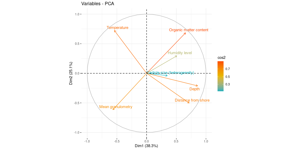
Figure 2: Overall distance-decay relationship and variation partitioning
env_data <- as.data.frame(as.matrix(ps_sed_norm@sam_data))
env_data <- env_data[ , c("Depth", "Shore_dist", "Horizon", "Temperature", "Water_mean", "MO_mean", "Dv43_mean", "dv_span_mean")]
# I don't include dv10, dv50, dv90 because strongly linked with Dv43

# adjust values to be numeric
levels(as.factor(env_data$Horizon))
## [1] "0_1" "1_3" "10_15" "15_30" "3_5" "30+" "5_10"
env_data$Horizon <- sub("0_1$", "1", env_data$Horizon)
env_data$Horizon <- sub("1_3$", "2", env_data$Horizon)
env_data$Horizon <- sub("3_5$", "3", env_data$Horizon)
env_data$Horizon <- sub("5_10$", "4", env_data$Horizon)
env_data$Horizon <- sub("10_15$", "5", env_data$Horizon)
env_data$Horizon <- sub("15_30$", "6", env_data$Horizon)
env_data$Horizon <- sub("30\\+$", "7", env_data$Horizon)

# let's remove samples missing environmental data
env_data <- env_data[is.na(env_data$Water_mean) == FALSE, ]
env_data <- env_data[is.na(env_data$MO_mean) == FALSE, ]
env_data <- env_data[is.na(env_data$Dv43_mean) == FALSE, ]
dim(env_data)
## [1] 183 8
# all columns must be of type numeric
env_data$Depth <- as.numeric(as.character(env_data$Depth))
env_data$Shore_dist <- as.numeric(as.character(env_data$Shore_dist))
env_data$Horizon <- as.numeric(as.character(env_data$Horizon))
env_data$Temperature <- as.numeric(as.character(env_data$Temperature))
env_data$Water_mean <- as.numeric(as.character(env_data$Water_mean))
env_data$MO_mean <- as.numeric(as.character(env_data$MO_mean))
env_data$Dv43_mean <- as.numeric(as.character(env_data$Dv43_mean))
env_data$dv_span_mean <- as.numeric(as.character(env_data$dv_span_mean))
# Geographical distance between communities
geo_df <- as.data.frame(as.matrix(ps_sed_norm@sam_data[,c("Longitude","Latitude")]))
geo_df$Longitude <- as.numeric(as.character(geo_df$Longitude))
geo_df$Latitude <- as.numeric(as.character(geo_df$Latitude))

# distance between the points in km
geo_distr <- pointDist(geo_df, distFunct=distVincentyEllipsoid, longLat = c("Longitude", "Latitude")) / 1000
rownames(geo_distr) <- rownames(geo_df)
colnames(geo_distr) <- rownames(geo_df)

min(geo_distr)
## [1] 0
max(geo_distr)
## [1] 7386.167
geo_dist <- geo_distr
# Bray-Curtis distance between communities
bc_dist <- vegdist(t(ps_sed_norm@otu_table), method = "bray")

# Bray-Curtis distance between communities as a function of geographical distance
bc_dist <- as.matrix(bc_dist)
class(geo_dist)

upper_tri_bc <- get_upper_tri(bc_dist)
melted_bc <- melt(upper_tri_bc, na.rm = TRUE)
colnames(melted_bc) <- c("Sample1", "Sample2", "BC_dist")

upper_tri_geo <- get_upper_tri(geo_dist)
melted_geo <- melt(upper_tri_geo, na.rm = TRUE)
colnames(melted_geo) <- c("Sample1", "Sample2", "Geo_dist")

df_distances <- merge(melted_bc, melted_geo)
# remove the diagonal (comparisons between same sample)
df_distances <- df_distances[df_distances$Sample1 != df_distances$Sample2,]

df_distances$Geo_dist_rel <- df_distances$Geo_dist/max(df_distances$Geo_dist)
df_distances$BC_sim <- (1 - df_distances$BC_dist)
df_distances$Log_bc_dist <- log(df_distances$BC_dist)

META <- data.frame(ps_sed_norm@sam_data)

df_distances$Sample1_zone = META[match(df_distances$Sample1, rownames(META)), "Geo_zone"]
df_distances$Sample2_zone = META[match(df_distances$Sample2, rownames(META)), "Geo_zone"]

df_distances$Sample1_horizon = META[match(df_distances$Sample1, rownames(META)), "Horizon"]
df_distances$Sample2_horizon = META[match(df_distances$Sample2, rownames(META)), "Horizon"]

# adding group
df_distances$Group[df_distances$Sample1_zone == "Atlantic_Ocean" & df_distances$Sample2_zone == "Atlantic_Ocean"] <- "Atlantic Ocean"
df_distances$Group[df_distances$Sample1_zone == "Transition" & df_distances$Sample2_zone == "Transition"] <- "Transition"
df_distances$Group[df_distances$Sample1_zone == "Mediterranean_Sea" & df_distances$Sample2_zone == "Mediterranean_Sea"] <- "Mediterranean Sea"

df_distances$Group[df_distances$Sample1_zone == "Atlantic_Ocean" & df_distances$Sample2_zone == "Transition"] <- "Atlantic - Transition"
df_distances$Group[df_distances$Sample1_zone == "Transition" & df_distances$Sample2_zone == "Atlantic_Ocean"] <- "Atlantic - Transition"

df_distances$Group[df_distances$Sample1_zone == "Atlantic_Ocean" & df_distances$Sample2_zone == "Mediterranean_Sea"] <- "Atlantic - Mediterranean"
df_distances$Group[df_distances$Sample1_zone == "Mediterranean_Sea" & df_distances$Sample2_zone == "Atlantic_Ocean"] <- "Atlantic - Mediterranean"

df_distances$Group[df_distances$Sample1_zone == "Mediterranean_Sea" & df_distances$Sample2_zone == "Transition"] <- "Mediterranean - Transition"
df_distances$Group[df_distances$Sample1_zone == "Transition" & df_distances$Sample2_zone == "Mediterranean_Sea"] <- "Mediterranean - Transition"

# Save this result and stop evaluating this chunk for faster knitting
saveRDS(df_distances, here::here("docs/Distance_decay_table_saved.rds"))
Log transforming dissimilarity values creates infinite values from 0.
Based on Martiny et al (2011), I replace 0 by the lowest similarity
value detected.
Here it is the comparison between AMIGO1_Site1_CT3_3-5 and
MDW_ST201_CT2_15-30 and is 2.953912e-06.
Considering that all the similarities that were calculated as 0 involve
heavily contaminated data that had to be severely cut into (Amigo
samples and Peacetime samples), it seems reasonable to set this value as
simply very low.
df_distances <- readRDS(here::here("docs/Distance_decay_table_saved.rds"))

df_distances[df_distances$BC_sim == min(df_distances[df_distances$BC_sim > 0, "BC_sim"]), ]
##                   Sample1             Sample2  BC_dist Geo_dist Geo_dist_rel
## 2536 AMIGO1_Site1_CT3_3-5 MDW_ST201_CT2_15-30 0.999997 3972.397    0.5378158
##            BC_sim   Log_bc_dist   Sample1_zone Sample2_zone Sample1_horizon
## 2536 2.953912e-06 -2.953916e-06 Atlantic_Ocean   Transition             3_5
##      Sample2_horizon                 Group
## 2536           15_30 Atlantic - Transition
df_distances$BC_sim[df_distances$BC_sim == 0] <- min(df_distances[df_distances$BC_sim > 0, "BC_sim"])
df_distances$Log_bc_sim <- log(df_distances$BC_sim)

df_distances$Group <- factor(df_distances$Group, levels = Group_order)
# centering environmental data
env_scaled <- scale(env_data, center = TRUE, scale = TRUE)
env_dist <- vegdist(env_scaled, method = "euclidean")
env_dist <- as.matrix(env_dist)

upper_tri_env <- get_upper_tri(env_dist)
melted_env <- reshape2::melt(upper_tri_env, na.rm = TRUE)
colnames(melted_env) <- c("Sample1", "Sample2", "Env_dist")

df_env <- merge(df_distances, melted_env)
df_env$Env_sim <- (1 - df_env$Env_dist)
Reducing comparisons to samples from the same horizon
df_distances <- df_distances[df_distances$Sample1_horizon == df_distances$Sample2_horizon, ]
df_distances$Horizon <- df_distances$Sample1_horizon
# with only log of bray-curtis, relative distance
lm_log_rel <- lm(df_distances$Log_bc_sim ~ df_distances$Geo_dist)
summary(lm_log_rel)
##
## Call:
## lm(formula = df_distances$Log_bc_sim ~ df_distances$Geo_dist)
##
## Residuals:
##     Min      1Q  Median      3Q     Max
## -5.7293 -0.7298  0.2585  1.0616  2.7008
##
## Coefficients:
##                         Estimate Std. Error t value Pr(>|t|)
## (Intercept)           -1.811e+00  3.309e-02  -54.72   <2e-16 ***
## df_distances$Geo_dist -4.911e-04  1.307e-05  -37.56   <2e-16 ***
## ---
## Signif. codes:  0 '***' 0.001 '**' 0.01 '*' 0.05 '.' 0.1 ' ' 1
##
## Residual standard error: 1.313 on 3852 degrees of freedom
## Multiple R-squared:  0.2681, Adjusted R-squared:  0.2679
## F-statistic:  1411 on 1 and 3852 DF,  p-value: < 2.2e-16
# Plotting for samples from the same region
df_distances_intra <- df_distances[df_distances$Group == "Atlantic Ocean" | df_distances$Group == "Transition" | df_distances$Group == "Mediterranean Sea",]

p2_1_intra <- ggplot(data = df_distances_intra, aes(x = Geo_dist, y = Log_bc_sim)) +
  geom_smooth(method = "lm", se=FALSE, formula = y~x) +
  geom_point() +
  stat_poly_eq(formula = y~x,
               aes(label = paste(..eq.label.., ..rr.label.., sep = "~~~")),
               parse = TRUE, label.x = "left", label.y = "bottom", size = 4)  +
  facet_wrap(~Group, nrow = 1, ncol = 3) + theme_1 +
  xlab("Geographic distance (km)") + ylab("Log(Bray-Curtis similarity)") +
  geom_abline(slope = lm_log_rel$coefficients[2], intercept = lm_log_rel$coefficients[1], color = "red")

# Plotting for samples from different regions
df_distances_inter <- df_distances[df_distances$Group != "Atlantic Ocean" & df_distances$Group != "Transition" & df_distances$Group != "Mediterranean Sea",]

p2_1_inter <- ggplot(data = df_distances_inter, aes(x = Geo_dist, y = Log_bc_sim)) +
  geom_smooth(method = "lm", se=FALSE, formula = y~x) +
  geom_point() +
  stat_poly_eq(formula = y~x,
               aes(label = paste(..eq.label.., ..rr.label.., sep = "~~~")),
               parse = TRUE, label.x = "left", label.y = "bottom", size = 4)  +
  facet_wrap(~Group, nrow = 1, ncol = 3) + theme_1 +
  xlab("Geographic distance (km)") + ylab("Log(Bray-Curtis similarity)") +
  geom_abline(slope = lm_log_rel$coefficients[2], intercept = lm_log_rel$coefficients[1], color = "red")
# p-value and stat for linear regressions of log(Bray-Curtis similarity) as a function of geographic distance by Group
# Results hidden for clarity
by(df_distances, df_distances$Group, function(x) summary(lm(x$Log_bc_sim ~ x$Geo_dist)))
df_env$Group <- factor(df_env$Group, levels = Group_order)
lm_env <- lm(df_env$BC_sim ~ df_env$Env_sim)
summary(lm_env)
##
## Call:
## lm(formula = df_env$BC_sim ~ df_env$Env_sim)
##
## Residuals:
##      Min       1Q   Median       3Q      Max
## -0.23668 -0.08957 -0.01924  0.05417  0.79650
##
## Coefficients:
##                 Estimate Std. Error t value Pr(>|t|)
## (Intercept)    0.2589835  0.0020484  126.43   <2e-16 ***
## df_env$Env_sim 0.0518730  0.0006619   78.36   <2e-16 ***
## ---
## Signif. codes:  0 '***' 0.001 '**' 0.01 '*' 0.05 '.' 0.1 ' ' 1
##
## Residual standard error: 0.1273 on 16651 degrees of freedom
## Multiple R-squared:  0.2694, Adjusted R-squared:  0.2694
## F-statistic:  6141 on 1 and 16651 DF,  p-value: < 2.2e-16
# Plotting for samples from the same region
df_env_intra <- df_env[df_env$Group == "Atlantic Ocean" | df_env$Group == "Transition" | df_env$Group == "Mediterranean Sea",]
dim(df_env_intra)
## [1] 5742 15
p2_2_intra <- ggplot(data = df_env_intra, aes(x = Env_sim, y = BC_sim)) +
  geom_smooth(method = "lm", se=FALSE, formula = y~x) +
  geom_point(alpha = 0.2) +
  stat_poly_eq(formula = y~x,
               aes(label = paste(..eq.label.., ..rr.label.., sep = "~~~")),
               parse = TRUE, label.x = "left", label.y = "top", size = 4)  +
  facet_wrap(~Group, nrow = 1, ncol = 3) + theme_1  + ylim(c(0, 0.8)) +
  xlab("Environmental similarity") + ylab("Bray-Curtis similarity") +
  geom_abline(slope = lm_env$coefficients[2], intercept = lm_env$coefficients[1], color = "red")

# Plotting for samples from different regions
df_env_inter <- df_env[df_env$Group != "Atlantic Ocean" & df_env$Group != "Transition" & df_env$Group != "Mediterranean Sea",]
dim(df_env_inter)
## [1] 10911 15
p2_2_inter <- ggplot(data = df_env_inter, aes(x = Env_sim, y = BC_sim)) +
  geom_smooth(method = "lm", se=FALSE, formula = y~x) +
  geom_point(alpha = 0.2) +
  stat_poly_eq(formula = y~x,
               aes(label = paste(..eq.label.., ..rr.label.., sep = "~~~")),
               parse = TRUE, label.x = "left", label.y = "top", size = 4)  +
  facet_wrap(~Group, nrow = 1, ncol = 3) + theme_1 + ylim(c(0, 0.8))+
  xlab("Environmental similarity") + ylab("Bray-Curtis similarity") +
  geom_abline(slope = lm_env$coefficients[2], intercept = lm_env$coefficients[1], color = "red")
# p-value and stat for linear regressions of Bray-curtis similarity as a function of environmental distance, by Group
# Results hidden for clarity
by(df_env, df_env$Group, function(x) summary(lm(x$BC_sim ~ x$Env_sim)))
# inside regions
p2_1_intra / p2_2_intra + plot_annotation(theme = theme_1)
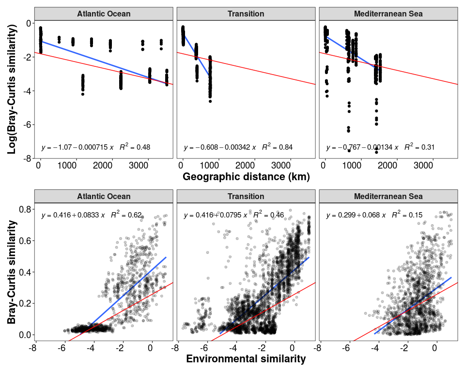
# between regions
p2_1_inter / p2_2_inter + plot_annotation(theme = theme_1)
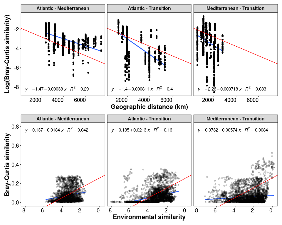
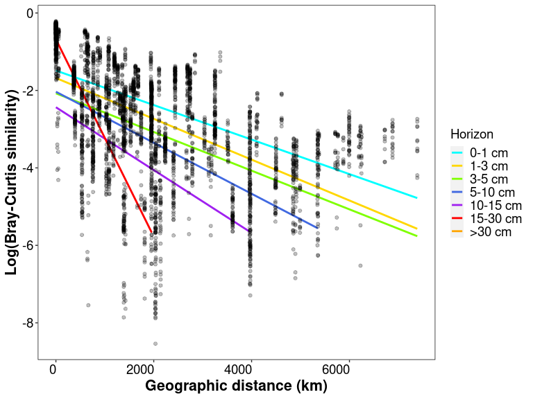
Figure 3: Evolution of the distance-decay with horizon depth
df_distances_01 <- subset(df_distances, df_distances$Horizon == "0_1")

df_distances_13 <- subset(df_distances, df_distances$Horizon == "1_3")

df_distances_35 <- subset(df_distances, df_distances$Horizon == "3_5")

df_distances_510 <- subset(df_distances, df_distances$Horizon == "5_10")

df_distances_1015 <- subset(df_distances, df_distances$Horizon == "10_15")

df_distances_1530 <- subset(df_distances, df_distances$Horizon == "15_30")

# Checking if the difference between slopes is signficant
d1 <- diffslope2(df_distances_01$Geo_dist, df_distances_01$Log_bc_sim, df_distances_13$Geo_dist, df_distances_13$Log_bc_sim, permutations = 1000)
c(d1$slope.diff, d1$signif)
## [1] 8.143906e-05 1.000000e-03
d1 <- diffslope2(df_distances_13$Geo_dist, df_distances_13$Log_bc_sim, df_distances_35$Geo_dist, df_distances_35$Log_bc_sim, permutations = 1000)
c(d1$slope.diff, d1$signif)
## [1] -2.779166e-05 6.000000e-02
d1 <- diffslope2(df_distances_35$Geo_dist, df_distances_35$Log_bc_sim, df_distances_510$Geo_dist, df_distances_510$Log_bc_sim, permutations = 1000)
c(d1$slope.diff, d1$signif)
## [1] 0.0001589592 0.0010000000
d1 <- diffslope2(df_distances_510$Geo_dist, df_distances_510$Log_bc_sim, df_distances_1015$Geo_dist, df_distances_1015$Log_bc_sim, permutations = 1000)
c(d1$slope.diff, d1$signif)
## [1] 0.0001525374 0.0060000000
d1 <- diffslope2(df_distances_1015$Geo_dist, df_distances_1015$Log_bc_sim, df_distances_1530$Geo_dist, df_distances_1530$Log_bc_sim, permutations = 1000)
c(d1$slope.diff, d1$signif)
## [1] 0.001737084 0.001000000
slope_horizon <- data.frame("Horizon" = c("0-1", "1-3", "3-5", "5-10", "10-15", "15-30"),
                            "Slope" = 0,
                            "Intersect" = 0,
                           "Adj_R_squared" = c(glance(lm(df_distances_01$Log_bc_sim ~ df_distances_01$Geo_dist))$adj.r.squared,
                                               glance(lm(df_distances_13$Log_bc_sim ~ df_distances_13$Geo_dist))$adj.r.squared,
                                               glance(lm(df_distances_35$Log_bc_sim ~ df_distances_35$Geo_dist))$adj.r.squared,
                                               glance(lm(df_distances_510$Log_bc_sim ~ df_distances_510$Geo_dist))$adj.r.squared,
                                               glance(lm(df_distances_1015$Log_bc_sim ~ df_distances_1015$Geo_dist))$adj.r.squared,
                                               glance(lm(df_distances_1530$Log_bc_sim ~ df_distances_1530$Geo_dist))$adj.r.squared))

slope_horizon$Slope[1] <- as.numeric(tidy(lm(df_distances_01$Log_bc_sim ~ df_distances_01$Geo_dist))[2,2])
slope_horizon$Slope[2] <- as.numeric(tidy(lm(df_distances_13$Log_bc_sim ~ df_distances_13$Geo_dist))[2,2])
slope_horizon$Slope[3] <- as.numeric(tidy(lm(df_distances_35$Log_bc_sim ~ df_distances_35$Geo_dist))[2,2])
slope_horizon$Slope[4] <- as.numeric(tidy(lm(df_distances_510$Log_bc_sim ~ df_distances_510$Geo_dist))[2,2])
slope_horizon$Slope[5] <- as.numeric(tidy(lm(df_distances_1015$Log_bc_sim ~ df_distances_1015$Geo_dist))[2,2])
slope_horizon$Slope[6] <- as.numeric(tidy(lm(df_distances_1530$Log_bc_sim ~ df_distances_1530$Geo_dist))[2,2])

slope_horizon$Intersect[1] <- as.numeric(tidy(lm(df_distances_01$Log_bc_sim ~ df_distances_01$Geo_dist))[1,2])
slope_horizon$Intersect[2] <- as.numeric(tidy(lm(df_distances_13$Log_bc_sim ~ df_distances_13$Geo_dist))[1,2])
slope_horizon$Intersect[3] <- as.numeric(tidy(lm(df_distances_35$Log_bc_sim ~ df_distances_35$Geo_dist))[1,2])
slope_horizon$Intersect[4] <- as.numeric(tidy(lm(df_distances_510$Log_bc_sim ~ df_distances_510$Geo_dist))[1,2])
slope_horizon$Intersect[5] <- as.numeric(tidy(lm(df_distances_1015$Log_bc_sim ~ df_distances_1015$Geo_dist))[1,2])
slope_horizon$Intersect[6] <- as.numeric(tidy(lm(df_distances_1530$Log_bc_sim ~ df_distances_1530$Geo_dist))[1,2])

slope_horizon$Horizon <- factor(slope_horizon$Horizon, levels = c("0-1", "1-3", "3-5", "5-10", "10-15", "15-30"))
slope_horizon
##   Horizon         Slope  Intersect Adj_R_squared
## 1     0-1 -0.0004457722 -1.4860418     0.3385871
## 2     1-3 -0.0005272112 -1.6785566     0.3995988
## 3     3-5 -0.0004994196 -2.0742524     0.2434741
## 4    5-10 -0.0006583787 -2.0343707     0.2900064
## 5   10-15 -0.0008109162 -2.4344533     0.1741814
## 6   15-30 -0.0025480005 -0.6796309     0.9671205
# plotting
lm_log_rel <- lm(df_distances$Log_bc_sim ~ df_distances$Geo_dist)

regressions <- ggplot(data = df_distances, aes(x = Geo_dist, y = Log_bc_sim)) +
  geom_smooth(method = "lm", se=FALSE, formula = y~x, aes(color = Horizon)) +
  geom_point(alpha = 0.25) +
  stat_poly_eq(formula = y~x,
               aes(label = paste("")),
               parse = TRUE, label.x = "right", label.y = "bottom", size = 3) + theme_1 +
  scale_colour_manual(labels = c("0-1 cm", "1-3 cm", "3-5 cm", "5-10 cm", "10-15 cm", "15-30 cm", ">30 cm"), values = scale_horizon) +
  xlab("Geographic distance (km)") + ylab("Log(Bray-Curtis similarity)")
regressions
# Linear models for DDR by horizon
# Results hidden for clarity
by(df_distances, df_distances$Horizon, function(x) summary(lm(x$Log_bc_sim ~ x$Geo_dist)))
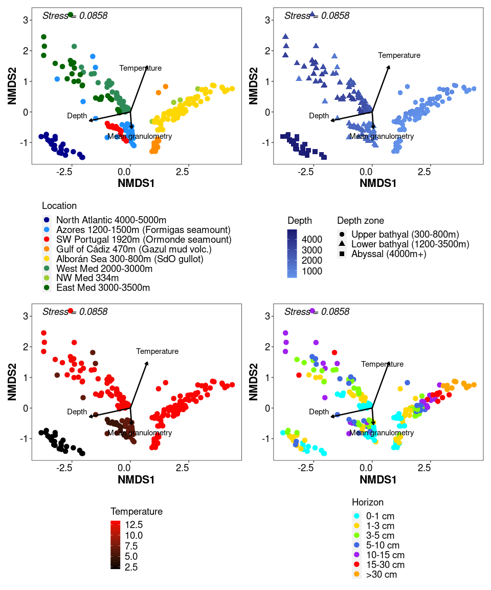
Figure 4: Ordinations (nMDS) and permanova
NMDS.ord <- ordinate(ps_sed_norm, "NMDS", "bray")
Based on the PCA, the environmental variables to be fitted here are:
Depth, Temperature, Granulometry, Humidity, Heterogeneity of particle
size.
Longitude and Latitude are correlated with Temperature, Distance from
shore is correlated with Depth + anti-correlated with Temp, Long, Lat.
Finally, OM is anti-correlated with granulometry.
## we can fit environmental variables onto unconstrained ordinations using envfit function in vegan.
# we can calculate the fit of the env. variables, and add the vectors as arrows:
fit <- envfit(NMDS.ord~Depth+Temperature+Water_mean+Dv43_mean+dv_span_mean,
              data = data.frame(ps_sed_norm@sam_data), permutations = how(nperm = 999), display = "sites", na.rm=T)
fit
##
## ***VECTORS
##
##                 NMDS1    NMDS2     r2 Pr(>r)
## Depth        -0.98674 -0.16233 0.7839  0.001 ***
## Temperature   0.43353  0.90114 0.6921  0.001 ***
## Water_mean   -0.47454 -0.88024 0.0101  0.392
## Dv43_mean     0.09830 -0.99516 0.0720  0.001 ***
## dv_span_mean -0.98650 -0.16378 0.0514  0.013 *
## ---
## Signif. codes:  0 '***' 0.001 '**' 0.01 '*' 0.05 '.' 0.1 ' ' 1
## Permutation: free
## Number of permutations: 999
##
## 25 observations deleted due to missingness
source ('https://raw.githubusercontent.com/zdealveindy/anadat-r/master/scripts/p.adjust.envfit.r')
ef.adj <- p.adjust.envfit (fit)
## Adjustment of significance by bonferroni method
ef.adj # humidity and heterogeneity are not significant
##
## ***VECTORS
##
##                 NMDS1    NMDS2     r2 Pr(>r)
## Depth        -0.98674 -0.16233 0.7839  0.005 **
## Temperature   0.43353  0.90114 0.6921  0.005 **
## Water_mean   -0.47454 -0.88024 0.0101  1.000
## Dv43_mean     0.09830 -0.99516 0.0720  0.005 **
## dv_span_mean -0.98650 -0.16378 0.0514  0.065 .
## ---
## Signif. codes:  0 '***' 0.001 '**' 0.01 '*' 0.05 '.' 0.1 ' ' 1
## Permutation: free
## Number of permutations: 999
##
## 25 observations deleted due to missingness
# plot arrows:
arrowmat = vegan::scores(fit, display = "bp")
# Add labels, make a data.frame
arrowdf <- data.frame(labels = rownames(arrowmat), arrowmat)
arrowdf = arrowdf[!arrowdf$labels %in% c("Water_mean", "dv_span_mean"),]
arrowdf$labels <- c("Depth", "Temperature", "Mean granulometry")

# Define the arrow aesthetic mapping
arrow_map = aes(xend = 2*NMDS1, yend = 2*NMDS2, x = 0, y = 0, shape = NULL, color = NULL, label = labels)
label_map = aes(x = 2.2 * NMDS1, y = 2.2 * NMDS2, shape = NULL, color = NULL, label = labels)
arrowhead = arrow(length = unit(0.02, "npc"))
library(ggrepel)
my_grob <-  grobTree(textGrob(paste("Stress =", as.character(signif(NMDS.ord$stress, 3))), x=0.05,  y=0.95, hjust=0, gp=gpar(col="Black", fontsize=14, fontface="italic")))

# nMDS bray-curtis colored by Location
sampleplot <-  plot_ordination(ps_sed_norm, NMDS.ord, type = "samples", color = "Location_depth")
f3_2 <- sampleplot + geom_point(size = 3) + theme_1 +
  scale_colour_manual(name="Location", values=scale_location) +  annotation_custom(my_grob) +
  theme(legend.position="bottom", legend.direction="vertical") +
  geom_segment(arrow_map, size = 0.9, data = arrowdf, color = "black", arrow = arrowhead) +
  geom_text_repel(label_map, size = 4, data = arrowdf, show.legend = F, point.padding = 1)

# nMDS bray-curtis colored by depth range
sampleplot <-  plot_ordination(ps_sed_norm, NMDS.ord, type = "samples", color = "Depth", shape = "Zone")
f3_3 <- sampleplot + geom_point(size = 3) + theme_1 +
  scale_colour_gradient(name="Depth", low = "cornflowerblue", high = "midnightblue") +
  scale_shape(name="Depth zone")+ annotation_custom(my_grob)+
  theme(legend.position="bottom", legend.direction="vertical") +
  geom_segment(arrow_map, size = 0.9, data = arrowdf, color = "black", arrow = arrowhead) +
  geom_text_repel(label_map, size = 4, data = arrowdf, show.legend = F, point.padding = 1)

# nMDS bray-curtis colored by temperature
sampleplot <-  plot_ordination(ps_sed_norm, NMDS.ord, type = "samples", color = "Temperature")
f3_4 <- sampleplot + geom_point(size = 3) + theme_1 + annotation_custom(my_grob) +
  scale_colour_gradient(name="Temperature", low = "black", high = "red") +
  theme(legend.position="bottom", legend.direction="vertical") +
  geom_segment(arrow_map, size = 0.9, data = arrowdf, color = "black", arrow = arrowhead) +
  geom_text_repel(label_map, size = 4, data = arrowdf, show.legend = F, point.padding = 1)

# NMDS bray-curtis colored by horizon
sampleplot <-  plot_ordination(ps_sed_norm, NMDS.ord, type = "samples", color = "Horizon")
f3_6 <- sampleplot + geom_point(size = 3) + theme_1 +
  scale_colour_manual(labels = c("0-1 cm", "1-3 cm", "3-5 cm", "5-10 cm", "10-15 cm", "15-30 cm", ">30 cm"), values = scale_horizon) + annotation_custom(my_grob) +
  theme(legend.position="bottom", legend.direction="vertical") +
  geom_segment(arrow_map, size = 0.9, data = arrowdf, color = "black", arrow = arrowhead) +
  geom_text_repel(label_map, size = 4, data = arrowdf, show.legend = F, point.padding = 1)

f3_2 + f3_3 + f3_4 + f3_6
Check dispersion of our unbalanced study
otu.table <- t(otu_table(ps_sed_norm))
sample_info <- data.frame(ps_sed_norm@sam_data)

# testing site
site.bd <- betadisper(dist, sample_info$Site)
anova(site.bd) # not significant
## Analysis of Variance Table
##
## Response: Distances
##            Df Sum Sq  Mean Sq F value  Pr(>F)
## Groups     19 0.5756 0.030295  1.5083 0.08612 .
## Residuals 190 3.8161 0.020085
## ---
## Signif. codes:  0 '***' 0.001 '**' 0.01 '*' 0.05 '.' 0.1 ' ' 1
# testing Horizon
horizon.bd <- betadisper(dist, sample_info$Horizon)
anova(horizon.bd)
## Analysis of Variance Table
##
## Response: Distances
##            Df Sum Sq  Mean Sq F value    Pr(>F)
## Groups      6 1.0665 0.177755  23.186 < 2.2e-16 ***
## Residuals 203 1.5563 0.007666
## ---
## Signif. codes:  0 '***' 0.001 '**' 0.01 '*' 0.05 '.' 0.1 ' ' 1
TukeyHSD(horizon.bd) # difference is significant when comparing 15-30 and 30+ to others
##   Tukey multiple comparisons of means
##     95% family-wise confidence level
##
## Fit: aov(formula = distances ~ group, data = df)
##
## $group
##                      diff         lwr         upr     p adj
## 1_3-0_1      0.0189907547 -0.03317208  0.07115358 0.9321499
## 3_5-0_1      0.0214249913 -0.03488684  0.07773682 0.9171884
## 5_10-0_1     0.0176968037 -0.04436503  0.07975864 0.9792856
## 10_15-0_1    0.0168829460 -0.04766526  0.08143116 0.9867420
## 15_30-0_1   -0.1636964950 -0.25038444 -0.07700855 0.0000013
## 30+-0_1     -0.2596937141 -0.34638166 -0.17300577 0.0000000
## 3_5-1_3      0.0024342366 -0.05435874  0.05922721 0.9999996
## 5_10-1_3    -0.0012939510 -0.06379267  0.06120477 1.0000000
## 10_15-1_3   -0.0021078087 -0.06707619  0.06286057 0.9999999
## 15_30-1_3   -0.1826872497 -0.26968850 -0.09568599 0.0000000
## 30+-1_3     -0.2786844689 -0.36568572 -0.19168321 0.0000000
## 5_10-3_5    -0.0037281875 -0.06972934  0.06227296 0.9999980
## 10_15-3_5   -0.0045420453 -0.07288641  0.06380232 0.9999949
## 15_30-3_5   -0.1851214863 -0.27467192 -0.09557105 0.0000001
## 30+-3_5     -0.2811187054 -0.37066914 -0.19156827 0.0000000
## 10_15-5_10  -0.0008138577 -0.07396849  0.07234078 1.0000000
## 15_30-5_10  -0.1813932987 -0.27466671 -0.08811989 0.0000005
## 30+-5_10    -0.2773905179 -0.37066393 -0.18411711 0.0000000
## 15_30-10_15 -0.1805794410 -0.27552537 -0.08563352 0.0000010
## 30+-10_15   -0.2765766602 -0.37152259 -0.18163073 0.0000000
## 30+-15_30   -0.0959972192 -0.20718650  0.01519206 0.1404512
# testing geographic zone
geo.bd <- betadisper(dist, sample_info$Geo_zone)
anova(geo.bd) # not significant
## Analysis of Variance Table
##
## Response: Distances
##            Df  Sum Sq   Mean Sq F value Pr(>F)
## Groups      2 0.01334 0.0066678  0.5382 0.5846
## Residuals 207 2.56458 0.0123893
Permanova tests
adonis2(otu.table~Site, data = sample_info, permutations = 999, method = "bray", by = "margin")
## Permutation test for adonis under NA model
## Marginal effects of terms
## Permutation: free
## Number of permutations: 999
##
## adonis2(formula = otu.table ~ Site, data = sample_info, permutations = 999, method = "bray", by = "margin")
##           Df SumOfSqs      R2      F Pr(>F)
## Site      19   44.320 0.51859 10.772  0.001 ***
## Residual 190   41.143 0.48141
## Total    209   85.463 1.00000
## ---
## Signif. codes:  0 '***' 0.001 '**' 0.01 '*' 0.05 '.' 0.1 ' ' 1
adonis2(otu.table~Geo_zone, data = sample_info, permutations = 999, method = "bray", by = "margin")
## Permutation test for adonis under NA model
## Marginal effects of terms
## Permutation: free
## Number of permutations: 999
##
## adonis2(formula = otu.table ~ Geo_zone, data = sample_info, permutations = 999, method = "bray", by = "margin")
##           Df SumOfSqs      R2      F Pr(>F)
## Geo_zone   2   15.732 0.18408 23.351  0.001 ***
## Residual 207   69.731 0.81592
## Total    209   85.463 1.00000
## ---
## Signif. codes:  0 '***' 0.001 '**' 0.01 '*' 0.05 '.' 0.1 ' ' 1
# here I should remove the deep horizons before doing this
# testing with block permutations for horizons since they are by site
perm <- how(nperm = 999)
setBlocks(perm) <- with(sample_info, Site)
adonis2(otu.table~Horizon, data = sample_info, permutations = perm,
        method = "bray", by = "margin", parallel = 15, na.action = na.exclude)
## Permutation test for adonis under NA model
## Marginal effects of terms
## Blocks:  with(sample_info, Site)
## Permutation: free
## Number of permutations: 999
##
## adonis2(formula = otu.table ~ Horizon, data = sample_info, permutations = perm, method = "bray", by = "margin", parallel = 15, na.action = na.exclude)
##           Df SumOfSqs      R2      F Pr(>F)
## Horizon    6   11.216 0.13124 5.1112  0.001 ***
## Residual 203   74.246 0.86876
## Total    209   85.463 1.00000
## ---
## Signif. codes:  0 '***' 0.001 '**' 0.01 '*' 0.05 '.' 0.1 ' ' 1
Figure 5: Local-scale analysis: DDR, correlation with environment, variation partitioning and biomarkers of horizon vs site
ps_alboran <- subset_samples(ps_sed, Location == "Alboran Sea (SdO gullot)")
ps_alboran <- prune_taxa(taxa_sums(ps_alboran)>0, ps_alboran)

# Re-establish full horizons and order
ps_alboran@sam_data$True_horizon <- ps_alboran@sam_data$Sample_ID
ps_alboran@sam_data$True_horizon <- gsub("MDW_ST..._CT._" , "", ps_alboran@sam_data$True_horizon)
ps_alboran@sam_data$True_horizon <- gsub("30_38|30_41|30_42|30_45|30_50", "30_40", ps_alboran@sam_data$True_horizon)
ps_alboran@sam_data$True_horizon <- factor(ps_alboran@sam_data$True_horizon,
                                           levels = c("0_1", "1_3", "3_5", "5_10", "10_15", "15_30", "30_40", "40_50"))
levels(as.factor(ps_alboran@sam_data$True_horizon))
## [1] "0_1" "1_3" "3_5" "5_10" "10_15" "15_30" "30_40" "40_50"
# Creating Surface and Subsurface sample categories with separation at 10 cmbsf
ps_alboran@sam_data$Horizon_category <- ps_alboran@sam_data$True_horizon
ps_alboran@sam_data$Horizon_category <- sub("0_1$|1_3|3_5|5_10", "Surface", ps_alboran@sam_data$Horizon_category)
ps_alboran@sam_data$Horizon_category <- sub("10_15|15_30|30_40|40_50", "Subsurface", ps_alboran@sam_data$Horizon_category)

# increase taxo for Proteobacteria
taxo <- data.frame(ps_alboran@tax_table)
taxo$Phylum_keep <- taxo$Phylum
taxo <- as.data.table(taxo)

# Make taxonomy clearer (see above)
taxo[Class=="Alphaproteobacteria", Phylum:="Proteobac.: Alphaproteobacteria"]
taxo[Class=="Gammaproteobacteria", Phylum:="Proteobac.: Gammaproteobacteria"]
taxo[Class=="Zetaproteobacteria", Phylum:="Proteobac.: Zetaproteobacteria"]
taxo[Class=="Magnetococcia", Phylum:="Proteobac.: Magnetococcia"]
taxo[Phylum=="Proteobacteria" & is.na(Class), Phylum:="Unassigned Proteobacteria"]
taxo[Class=="Bathyarchaeia", Phylum:="Crenarchaeota: Bathyarchaeia"]
taxo[Class=="Nitrososphaeria", Phylum:="Crenarchaeota: Nitrososphaeria"]
taxo[Phylum=="Crenarchaeota", Phylum:="Crenarchaeota (NA)"]

taxo <- as.matrix(taxo)
rownames(taxo) <- taxa_names(ps_alboran)
ps_alboran <- phyloseq(otu_table(ps_alboran), tax_table(taxo), sample_data(ps_alboran))
Overall biomarkers of subsurface
# start with raw data, not normalized
deseq <- ps_alboran
deseq <-  phyloseq_to_deseq2(deseq, ~ Horizon_category)
deseq$Horizon_category <- factor(deseq$Horizon_category, levels = c("Surface", "Subsurface"))

geoMeans <- apply(counts(deseq), 1, gm_mean)
deseq <- estimateSizeFactors(deseq, geoMeans = geoMeans)
deseq <- DESeq(deseq, fitType="local")
res <- results(deseq)
summary(res)
##
## out of 116763 with nonzero total read count
## adjusted p-value < 0.1
## LFC > 0 (up)       : 5654, 4.8%
## LFC < 0 (down)     : 5182, 4.4%
## outliers [1]       : 0, 0%
## low counts [2]     : 108855, 93%
## (mean count < 1)
## [1] see 'cooksCutoff' argument of ?results
## [2] see 'independentFiltering' argument of ?results
# Keep only significant
resSub <- subset(res, padj < 0.01)

Sub <- as.data.frame(resSub)
df <- cbind(taxa = rownames(Sub), Sub)
df$taxa <- c(1:nrow(df))

setorder(df, log2FoldChange)
overall_surface_taxa <- df[df$log2FoldChange < 0, ]
overall_subsurface_taxa <- df[df$log2FoldChange > 0, ]
Let’s compute biomarkers for each site, using only the surface horizons.
ps_alboran_surface <- subset_samples(ps_alboran, Horizon_category == "Surface")
ps_alboran_surface <- prune_taxa(taxa_sums(ps_alboran_surface)>0, ps_alboran_surface)
ps_alboran_surface
## phyloseq-class experiment-level object
## otu_table()   OTU Table:         [ 73292 taxa and 36 samples ]
## sample_data() Sample Data:       [ 36 samples by 30 sample variables ]
## tax_table()   Taxonomy Table:    [ 73292 taxa by 15 taxonomic ranks ]
ps_alboran_surface@sam_data$Site_215 <- ps_alboran_surface@sam_data$Site
ps_alboran_surface@sam_data$Site_215 <- gsub("MDW_ST201", "Other", ps_alboran_surface@sam_data$Site_215)
ps_alboran_surface@sam_data$Site_215 <- gsub("MDW_ST179", "Other", ps_alboran_surface@sam_data$Site_215)

ps_alboran_surface@sam_data$Site_201 <- ps_alboran_surface@sam_data$Site
ps_alboran_surface@sam_data$Site_201 <- gsub("MDW_ST215", "Other", ps_alboran_surface@sam_data$Site_201)
ps_alboran_surface@sam_data$Site_201 <- gsub("MDW_ST179", "Other", ps_alboran_surface@sam_data$Site_201)

ps_alboran_surface@sam_data$Site_179 <- ps_alboran_surface@sam_data$Site
ps_alboran_surface@sam_data$Site_179 <- gsub("MDW_ST201", "Other", ps_alboran_surface@sam_data$Site_179)
ps_alboran_surface@sam_data$Site_179 <- gsub("MDW_ST215", "Other", ps_alboran_surface@sam_data$Site_179)
Biomarkers of site 215 compared to other sites
# start with raw data, not normalized
deseq <- ps_alboran_surface
deseq <-  phyloseq_to_deseq2(deseq, ~ Site_215)
deseq$Site_215 <- factor(deseq$Site_215, levels = c("MDW_ST215", "Other"))

geoMeans <- apply(counts(deseq), 1, gm_mean)
deseq <- estimateSizeFactors(deseq, geoMeans = geoMeans)
deseq <- DESeq(deseq, fitType="local")
res <- results(deseq)
summary(res)
##
## out of 62533 with nonzero total read count
## adjusted p-value < 0.1
## LFC > 0 (up)       : 107, 0.17%
## LFC < 0 (down)     : 35, 0.056%
## outliers [1]       : 0, 0%
## low counts [2]     : 10759, 17%
## (mean count < 0)
## [1] see 'cooksCutoff' argument of ?results
## [2] see 'independentFiltering' argument of ?results
resSub <- subset(res, padj < 0.01)

Sub <- as.data.frame(resSub)
df <- cbind(taxa = rownames(Sub), Sub)
df$taxa <- c(1:nrow(df))

setorder(df, log2FoldChange)
biomarker_215 <- df[df$log2FoldChange < 0, ]
Biomarkers of site 201 compared to other sites
# start with raw data, not normalized
deseq <- ps_alboran_surface
deseq <-  phyloseq_to_deseq2(deseq, ~ Site_201)
deseq$Site_201 <- factor(deseq$Site_201, levels = c("MDW_ST201", "Other"))

geoMeans <- apply(counts(deseq), 1, gm_mean)
deseq <- estimateSizeFactors(deseq, geoMeans = geoMeans)
deseq <- DESeq(deseq, fitType="local")
res <- results(deseq)
summary(res)
##
## out of 62699 with nonzero total read count
## adjusted p-value < 0.1
## LFC > 0 (up)       : 1112, 1.8%
## LFC < 0 (down)     : 207, 0.33%
## outliers [1]       : 0, 0%
## low counts [2]     : 63603, 101%
## (mean count < 3)
## [1] see 'cooksCutoff' argument of ?results
## [2] see 'independentFiltering' argument of ?results
resSub <- subset(res, padj < 0.01)

Sub <- as.data.frame(resSub)
df <- cbind(taxa = rownames(Sub), Sub)
df$taxa <- c(1:nrow(df))

setorder(df, log2FoldChange)
biomarker_201 <- df[df$log2FoldChange < 0, ]
Biomarkers of site 179 compared to other sites
# start with raw data, not normalized
deseq <- ps_alboran_surface
deseq <-  phyloseq_to_deseq2(deseq, ~ Site_179)
deseq$Site_179 <- factor(deseq$Site_179, levels = c("MDW_ST179", "Other"))

geoMeans <- apply(counts(deseq), 1, gm_mean)
deseq <- estimateSizeFactors(deseq, geoMeans = geoMeans)
deseq <- DESeq(deseq, fitType="local")
res <- results(deseq)
summary(res)
##
## out of 62683 with nonzero total read count
## adjusted p-value < 0.1
## LFC > 0 (up)       : 1228, 2%
## LFC < 0 (down)     : 704, 1.1%
## outliers [1]       : 0, 0%
## low counts [2]     : 58787, 94%
## (mean count < 1)
## [1] see 'cooksCutoff' argument of ?results
## [2] see 'independentFiltering' argument of ?results
resSub <- subset(res, padj < 0.01)

Sub <- as.data.frame(resSub)
df <- cbind(taxa = rownames(Sub), Sub)
df$taxa <- c(1:nrow(df))

setorder(df, log2FoldChange)
biomarker_179 <- df[df$log2FoldChange < 0, ]
Creating phyloseq objects by site, and by horizon category at each site
# these objects are count data without singletons
ps_201 <- subset_samples(ps_alboran, Site == "MDW_ST201")
ps_201 <- prune_taxa(taxa_sums(ps_201)>0, ps_201)

ps_215 <- subset_samples(ps_alboran, Site == "MDW_ST215")
ps_215 <- prune_taxa(taxa_sums(ps_215)>0, ps_215)

ps_179 <- subset_samples(ps_alboran, Site == "MDW_ST179")
ps_179 <- prune_taxa(taxa_sums(ps_179)>0, ps_179)
ps_179_subsurface <- subset_samples(ps_179, Horizon_category == "Subsurface")
ps_179_subsurface <- prune_taxa(taxa_sums(ps_179_subsurface)>0, ps_179_subsurface)

ps_201_subsurface <- subset_samples(ps_201, Horizon_category == "Subsurface")
ps_201_subsurface <- prune_taxa(taxa_sums(ps_201_subsurface)>0, ps_201_subsurface)

ps_215_subsurface <- subset_samples(ps_215, Horizon_category == "Subsurface")
ps_215_subsurface <- prune_taxa(taxa_sums(ps_215_subsurface)>0, ps_215_subsurface)

ps_179_surface <- subset_samples(ps_179, Horizon_category == "Surface")
ps_179_surface <- prune_taxa(taxa_sums(ps_179_surface)>0, ps_179_surface)

ps_201_surface <- subset_samples(ps_201, Horizon_category == "Surface")
ps_201_surface <- prune_taxa(taxa_sums(ps_201_surface)>0, ps_201_surface)

ps_215_surface <- subset_samples(ps_215, Horizon_category == "Surface")
ps_215_surface <- prune_taxa(taxa_sums(ps_215_surface)>0, ps_215_surface)
Making dataframe of the composition of the surface communities at each site, based on the biomarker detection
df_surface <- data.frame("Site" = c("MDW_ST201", "MDW_ST215", "MDW_ST179"),
                           "Site_biomarkers" = 0,
                           "Surface_biomarkers" = 0,
                           "Subsurface_biomarkers" = 0,
                           "Unexplained" = 0)

# Site 179
df_surface[df_surface$Site == "MDW_ST179", "Site_biomarkers"] <-
  signif((sum(sample_sums(prune_taxa(taxa_names(ps_179_surface) %in% rownames(biomarker_179), ps_179_surface))) / sum(sample_sums(ps_179_surface)) * 100), 3)
df_surface[df_surface$Site == "MDW_ST179", "Subsurface_biomarkers"] <-
  signif((sum(sample_sums(prune_taxa(taxa_names(ps_179_surface) %in% rownames(overall_subsurface_taxa), ps_179_surface))) / sum(sample_sums(ps_179_surface)) * 100), 3)
df_surface[df_surface$Site == "MDW_ST179", "Surface_biomarkers"] <-
  signif((sum(sample_sums(prune_taxa(taxa_names(ps_179_surface) %in% rownames(overall_surface_taxa), ps_179_surface))) / sum(sample_sums(ps_179_surface)) * 100), 3)

unexplained_179 <- setdiff(taxa_names(ps_179_surface), unique(c(rownames(biomarker_179), rownames(overall_subsurface_taxa), rownames(overall_surface_taxa))))

df_surface[df_surface$Site == "MDW_ST179", "Unexplained"] <-
  signif((sum(sample_sums(prune_taxa(taxa_names(ps_179_surface) %in% unexplained_179, ps_179_surface))) / sum(sample_sums(ps_179_surface)) * 100), 3)

# Site 201
df_surface[df_surface$Site == "MDW_ST201", "Site_biomarkers"] <-
  signif((sum(sample_sums(prune_taxa(taxa_names(ps_201_surface) %in% rownames(biomarker_201), ps_201_surface))) / sum(sample_sums(ps_201_surface)) * 100), 3)
df_surface[df_surface$Site == "MDW_ST201", "Subsurface_biomarkers"] <-
  signif((sum(sample_sums(prune_taxa(taxa_names(ps_201_surface) %in% rownames(overall_subsurface_taxa), ps_201_surface))) / sum(sample_sums(ps_201_surface)) * 100), 3)
df_surface[df_surface$Site == "MDW_ST201", "Surface_biomarkers"] <-
  signif((sum(sample_sums(prune_taxa(taxa_names(ps_201_surface) %in% rownames(overall_surface_taxa), ps_201_surface))) / sum(sample_sums(ps_201_surface)) * 100), 3)

unexplained_201 <- setdiff(taxa_names(ps_201_surface), unique(c(rownames(biomarker_201), rownames(overall_subsurface_taxa), rownames(overall_surface_taxa))))

df_surface[df_surface$Site == "MDW_ST201", "Unexplained"] <-
  signif((sum(sample_sums(prune_taxa(taxa_names(ps_201_surface) %in% unexplained_201, ps_201_surface))) / sum(sample_sums(ps_201_surface)) * 100), 3)

# Site 215
df_surface[df_surface$Site == "MDW_ST215", "Site_biomarkers"] <-
  signif((sum(sample_sums(prune_taxa(taxa_names(ps_215_surface) %in% rownames(biomarker_215), ps_215_surface))) / sum(sample_sums(ps_215_surface)) * 100), 3)
df_surface[df_surface$Site == "MDW_ST215", "Subsurface_biomarkers"] <-
  signif((sum(sample_sums(prune_taxa(taxa_names(ps_215_surface) %in% rownames(overall_subsurface_taxa), ps_215_surface))) / sum(sample_sums(ps_215_surface)) * 100), 3)
df_surface[df_surface$Site == "MDW_ST215", "Surface_biomarkers"] <-
  signif((sum(sample_sums(prune_taxa(taxa_names(ps_215_surface) %in% rownames(overall_surface_taxa), ps_215_surface))) / sum(sample_sums(ps_215_surface)) * 100), 3)

unexplained_215 <- setdiff(taxa_names(ps_215_surface), unique(c(rownames(biomarker_215), rownames(overall_subsurface_taxa), rownames(overall_surface_taxa))))

df_surface[df_surface$Site == "MDW_ST215", "Unexplained"] <-
  signif((sum(sample_sums(prune_taxa(taxa_names(ps_215_surface) %in% unexplained_215, ps_215_surface))) / sum(sample_sums(ps_215_surface)) * 100), 3)

df_surface
##        Site Site_biomarkers Surface_biomarkers Subsurface_biomarkers
## 1 MDW_ST201           1.660               45.8                  2.13
## 2 MDW_ST215           0.343               42.8                  2.43
## 3 MDW_ST179           4.320               38.5                  1.91
##   Unexplained
## 1        51.6
## 2        54.4
## 3        56.9
melt_df_surface <- melt(df_surface)
colnames(melt_df_surface) <- c("Site", "Category", "Percent_of_comm")

# plot as stacked bar
a <- ggplot(melt_df_surface, aes(x = Site, y = Percent_of_comm, fill = Category)) +
  geom_bar(stat = "identity", position = "stack") +
  theme(axis.text.x = element_text(size = 12, angle = 0),
        axis.title.x = element_blank(),
        axis.text.y = element_text(size = 12),
        axis.title.y = element_text(size = 14),
        legend.position="bottom",
        legend.title = element_blank(),
        legend.text = element_text(size = 14),
        plot.title = element_text(size = 18, hjust = 0.5)) +
  coord_flip() +
  ggtitle("Surface communities by site")
Making dataframe of the composition of the subsurface communities at each site, based on the biomarker detection
df_subsurface <- data.frame("Site" = c("MDW_ST201", "MDW_ST215", "MDW_ST179"),
                           "Site_biomarkers" = 0,
                           "Surface_biomarkers" = 0,
                           "Subsurface_biomarkers" = 0,
                           "Unexplained" = 0)

# Site 179
df_subsurface[df_subsurface$Site == "MDW_ST179", "Site_biomarkers"] <-
  signif((sum(sample_sums(prune_taxa(taxa_names(ps_179_subsurface) %in% rownames(biomarker_179), ps_179_subsurface))) / sum(sample_sums(ps_179_subsurface)) * 100), 3)
df_subsurface[df_subsurface$Site == "MDW_ST179", "Subsurface_biomarkers"] <-
  signif((sum(sample_sums(prune_taxa(taxa_names(ps_179_subsurface) %in% rownames(overall_subsurface_taxa), ps_179_subsurface))) / sum(sample_sums(ps_179_subsurface)) * 100), 3)
df_subsurface[df_subsurface$Site == "MDW_ST179", "Surface_biomarkers"] <-
  signif((sum(sample_sums(prune_taxa(taxa_names(ps_179_subsurface) %in% rownames(overall_surface_taxa), ps_179_subsurface))) / sum(sample_sums(ps_179_subsurface)) * 100), 3)

unexplained_179 <- setdiff(taxa_names(ps_179_subsurface), unique(c(rownames(biomarker_179), rownames(overall_subsurface_taxa), rownames(overall_surface_taxa))))

df_subsurface[df_subsurface$Site == "MDW_ST179", "Unexplained"] <-
  signif((sum(sample_sums(prune_taxa(taxa_names(ps_179_subsurface) %in% unexplained_179, ps_179_subsurface))) / sum(sample_sums(ps_179_subsurface)) * 100), 3)

# Site 201
df_subsurface[df_subsurface$Site == "MDW_ST201", "Site_biomarkers"] <-
  signif((sum(sample_sums(prune_taxa(taxa_names(ps_201_subsurface) %in% rownames(biomarker_201), ps_201_subsurface))) / sum(sample_sums(ps_201_subsurface)) * 100), 3)
df_subsurface[df_subsurface$Site == "MDW_ST201", "Subsurface_biomarkers"] <-
  signif((sum(sample_sums(prune_taxa(taxa_names(ps_201_subsurface) %in% rownames(overall_subsurface_taxa), ps_201_subsurface))) / sum(sample_sums(ps_201_subsurface)) * 100), 3)
df_subsurface[df_subsurface$Site == "MDW_ST201", "Surface_biomarkers"] <-
  signif((sum(sample_sums(prune_taxa(taxa_names(ps_201_subsurface) %in% rownames(overall_surface_taxa), ps_201_subsurface))) / sum(sample_sums(ps_201_subsurface)) * 100), 3)

unexplained_201 <- setdiff(taxa_names(ps_201_subsurface), unique(c(rownames(biomarker_201), rownames(overall_subsurface_taxa), rownames(overall_surface_taxa))))

df_subsurface[df_subsurface$Site == "MDW_ST201", "Unexplained"] <-
  signif((sum(sample_sums(prune_taxa(taxa_names(ps_201_subsurface) %in% unexplained_201, ps_201_subsurface))) / sum(sample_sums(ps_201_subsurface)) * 100), 3)

# Site 215
df_subsurface[df_subsurface$Site == "MDW_ST215", "Site_biomarkers"] <-
  signif((sum(sample_sums(prune_taxa(taxa_names(ps_215_subsurface) %in% rownames(biomarker_215), ps_215_subsurface))) / sum(sample_sums(ps_215_subsurface)) * 100), 3)
df_subsurface[df_subsurface$Site == "MDW_ST215", "Subsurface_biomarkers"] <-
  signif((sum(sample_sums(prune_taxa(taxa_names(ps_215_subsurface) %in% rownames(overall_subsurface_taxa), ps_215_subsurface))) / sum(sample_sums(ps_215_subsurface)) * 100), 3)
df_subsurface[df_subsurface$Site == "MDW_ST215", "Surface_biomarkers"] <-
  signif((sum(sample_sums(prune_taxa(taxa_names(ps_215_subsurface) %in% rownames(overall_surface_taxa), ps_215_subsurface))) / sum(sample_sums(ps_215_subsurface)) * 100), 3)

unexplained_215 <- setdiff(taxa_names(ps_215_subsurface), unique(c(rownames(biomarker_215), rownames(overall_subsurface_taxa), rownames(overall_surface_taxa))))

df_subsurface[df_subsurface$Site == "MDW_ST215", "Unexplained"] <-
  signif((sum(sample_sums(prune_taxa(taxa_names(ps_215_subsurface) %in% unexplained_215, ps_215_subsurface))) / sum(sample_sums(ps_215_subsurface)) * 100), 3)

df_subsurface
##        Site Site_biomarkers Surface_biomarkers Subsurface_biomarkers
## 1 MDW_ST201           0.625               5.37                  43.3
## 2 MDW_ST215           0.306               5.82                  38.8
## 3 MDW_ST179           1.450               3.27                  44.1
##   Unexplained
## 1        51.1
## 2        55.0
## 3        51.6
melt_df_subsurface <- melt(df_subsurface)
colnames(melt_df_subsurface) <- c("Site", "Category", "Percent_of_comm")

# plot as stacked bar
b <- ggplot(melt_df_subsurface, aes(x = Site, y = Percent_of_comm, fill = Category)) +
  geom_bar(stat = "identity", position = "stack") +
  theme(axis.text.x = element_text(size = 12, angle = 0),
        axis.title.x = element_blank(),
        axis.text.y = element_text(size = 12),
        axis.title.y = element_text(size = 14),
        legend.position="bottom",
        legend.title = element_blank(),
        legend.text = element_text(size = 14),
        plot.title = element_text(size = 18, hjust = 0.5)) +
  coord_flip() +
  ggtitle("Subsurface communities by site")

a+b + plot_layout(guides = "collect") & theme(legend.position="bottom")
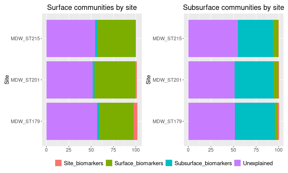
Evolution of Bray-Curtis similarity with geographic and environmental distances
Subsampling distance dataframes
df_distances_4 <- subset(df_distances, grepl("MDW_ST201|MDW_ST215|MDW_ST179", df_distances$Sample1) &
                           grepl("MDW_ST201|MDW_ST215|MDW_ST179", df_distances$Sample2))

df_env_4 <- subset(df_env, grepl("MDW_ST201|MDW_ST215|MDW_ST179", df_env$Sample1) &
                           grepl("MDW_ST201|MDW_ST215|MDW_ST179", df_env$Sample2))
lm_log_rel <- lm(df_distances_4$Log_bc_sim ~ df_distances_4$Geo_dist)
summary(lm(df_distances_4$Log_bc_sim ~ df_distances_4$Geo_dist))
##
## Call:
## lm(formula = df_distances_4$Log_bc_sim ~ df_distances_4$Geo_dist)
##
## Residuals:
##      Min       1Q   Median       3Q      Max
## -0.53313 -0.06307  0.03986  0.09287  0.25864
##
## Coefficients:
##                          Estimate Std. Error t value Pr(>|t|)
## (Intercept)             -0.441250   0.014858  -29.70   <2e-16 ***
## df_distances_4$Geo_dist -0.030863   0.002014  -15.33   <2e-16 ***
## ---
## Signif. codes:  0 '***' 0.001 '**' 0.01 '*' 0.05 '.' 0.1 ' ' 1
##
## Residual standard error: 0.1433 on 269 degrees of freedom
## Multiple R-squared:  0.4661, Adjusted R-squared:  0.4642
## F-statistic: 234.9 on 1 and 269 DF,  p-value: < 2.2e-16
p <- ggplot(data = df_distances_4, aes(x = Geo_dist, y = Log_bc_sim)) +
  geom_smooth(method = "lm", se=FALSE, formula = y~x, aes(color = Horizon)) +
  geom_point() +
  stat_poly_eq(formula = y~x,
               aes(label = paste(""), color = Horizon),
               parse = TRUE, label.x = "left", label.y = "bottom", size = 3)  + theme_1 +
  scale_colour_manual(labels = c("0-1 cm", "1-3 cm", "3-5 cm", "5-10 cm", "10-15 cm", "15-30 cm", ">30 cm"), values = scale_horizon) +
  xlab("Geographic distance (km)") + ylab("Log(Bray-Curtis similarity)")
p
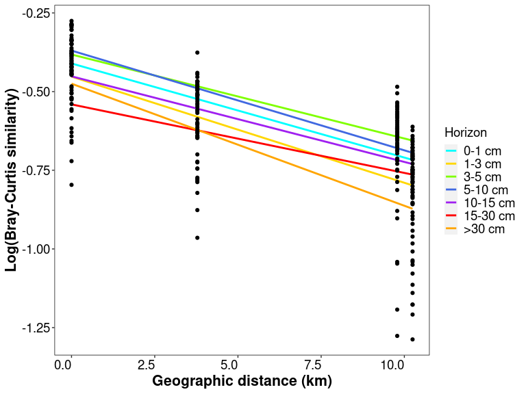
# hidden for clarity
by(df_distances_4, df_distances_4$Horizon, function(x) summary(lm(x$Log_bc_sim ~ x$Geo_dist)))
summary(lm(df_env_4$BC_sim ~ df_env_4$Env_sim))
##
## Call:
## lm(formula = df_env_4$BC_sim ~ df_env_4$Env_sim)
##
## Residuals:
##      Min       1Q   Median       3Q      Max
## -0.24116 -0.07645 -0.00484  0.07240  0.39330
##
## Coefficients:
##                  Estimate Std. Error t value Pr(>|t|)
## (Intercept)      0.498582   0.003742   133.2   <2e-16 ***
## df_env_4$Env_sim 0.116261   0.003036    38.3   <2e-16 ***
## ---
## Signif. codes:  0 '***' 0.001 '**' 0.01 '*' 0.05 '.' 0.1 ' ' 1
##
## Residual standard error: 0.1025 on 1273 degrees of freedom
## Multiple R-squared:  0.5354, Adjusted R-squared:  0.535
## F-statistic:  1467 on 1 and 1273 DF,  p-value: < 2.2e-16
q <- ggplot(data = df_env_4, aes(x = Env_sim, y = BC_sim)) +
  geom_smooth(method = "lm", se=FALSE, formula = y~x) +
  geom_point(alpha = 0.25) +
  stat_poly_eq(formula = y~x,
               aes(label = paste(..eq.label.., ..rr.label.., sep = "~~~")),
               parse = TRUE, label.x = "left", label.y = "top", size = 7) +
  theme_1 +
  xlab("Environmental similarity") + ylab("Bray-Curtis similarity") +
  geom_abline(slope = lm_env$coefficients[2], intercept = lm_env$coefficients[1], color = "red")
q
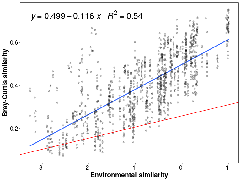
Variation partitioning at local scale
ps_sed_varpart <- prune_samples(intersect(sample_names(ps_sed_norm), rownames(env_data)), ps_sed_norm)
ps_sed_varpart <- subset_samples(ps_sed_varpart, Location == "Alboran Sea (SdO gullot)")
ps_sed_varpart <- prune_taxa(taxa_sums(ps_sed_varpart) > 0, ps_sed_varpart)

geo_df_short <- as.data.frame(as.matrix(ps_sed_varpart@sam_data[,c("Longitude","Latitude")]))
geo_df_short$Longitude <- as.numeric(as.character(geo_df_short$Longitude))
geo_df_short$Latitude <- as.numeric(as.character(geo_df_short$Latitude))
geo_df_short$X2 <- geo_df_short$Latitude^2

env_short <- env_data[intersect(sample_names(ps_sed_varpart), rownames(env_data)), ]
env_short$Temperature <- NULL

bc_dist <- vegdist(t(ps_sed_varpart@otu_table), method = "bray")

var.part2 <- varpart(bc_dist, env_short[,"Depth"], env_short[,"Horizon"])
showvarparts(2,labels=as.character(round(var.part2$part$indfract$Adj.R.square, 3)*100),
             bg=c("blue","red"), Xnames = c("Site","Horizon"))
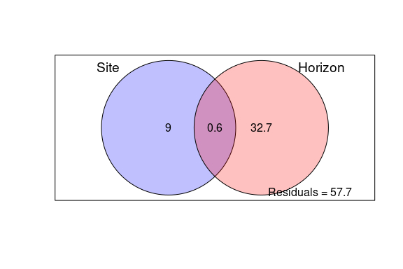
# testing significance
rda.all <- dbrda(bc_dist~Depth+Horizon, data = env_short)
anova(rda.all)
## Permutation test for dbrda under reduced model
## Permutation: free
## Number of permutations: 999
##
## Model: dbrda(formula = bc_dist ~ Depth + Horizon, data = env_short)
##          Df SumOfSqs      F Pr(>F)
## Model     2   4.1770 19.321  0.001 ***
## Residual 48   5.1885
## ---
## Signif. codes:  0 '***' 0.001 '**' 0.01 '*' 0.05 '.' 0.1 ' ' 1
rda.depth <- dbrda (bc_dist~Depth, data = env_short)
anova(rda.depth)
## Permutation test for dbrda under reduced model
## Permutation: free
## Number of permutations: 999
##
## Model: dbrda(formula = bc_dist ~ Depth, data = env_short)
##          Df SumOfSqs      F Pr(>F)
## Model     1   1.0674 6.3027  0.001 ***
## Residual 49   8.2982
## ---
## Signif. codes:  0 '***' 0.001 '**' 0.01 '*' 0.05 '.' 0.1 ' ' 1
rda.horizon <- dbrda (bc_dist~Horizon, data = env_short)
anova(rda.horizon)
## Permutation test for dbrda under reduced model
## Permutation: free
## Number of permutations: 999
##
## Model: dbrda(formula = bc_dist ~ Horizon, data = env_short)
##          Df SumOfSqs      F Pr(>F)
## Model     1   3.2401 25.919  0.001 ***
## Residual 49   6.1254
## ---
## Signif. codes:  0 '***' 0.001 '**' 0.01 '*' 0.05 '.' 0.1 ' ' 1
rda.depth.horizon <- dbrda (bc_dist~Depth + Condition(Horizon), data = env_short)
anova(rda.depth.horizon)
## Permutation test for dbrda under reduced model
## Permutation: free
## Number of permutations: 999
##
## Model: dbrda(formula = bc_dist ~ Depth + Condition(Horizon), data = env_short)
##          Df SumOfSqs      F Pr(>F)
## Model     1   0.9369 8.6673  0.001 ***
## Residual 48   5.1885
## ---
## Signif. codes:  0 '***' 0.001 '**' 0.01 '*' 0.05 '.' 0.1 ' ' 1
rda.horizon.depth <- dbrda (bc_dist~Horizon + Condition(Depth), data = env_short)
anova(rda.horizon.depth)
## Permutation test for dbrda under reduced model
## Permutation: free
## Number of permutations: 999
##
## Model: dbrda(formula = bc_dist ~ Horizon + Condition(Depth), data = env_short)
##          Df SumOfSqs      F Pr(>F)
## Model     1   3.1096 28.768  0.001 ***
## Residual 48   5.1885
## ---
## Signif. codes:  0 '***' 0.001 '**' 0.01 '*' 0.05 '.' 0.1 ' ' 1
var.part2 <- varpart(bc_dist, env_short[,"Water_mean"] + env_short[,"MO_mean"] + env_short[,"Dv43_mean"] + env_short[,"dv_span_mean"],
                     env_short[,"Horizon"])
showvarparts(2,labels=as.character(round(var.part2$part$indfract$Adj.R.square, 3)*100), bg=c("green","red"), Xnames = c("Sedimentary char.","Horizon"))
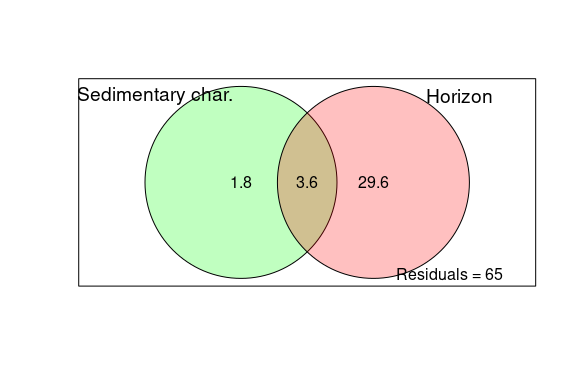
# testing significance
rda.all <- dbrda(bc_dist~Water_mean+MO_mean+Dv43_mean+dv_span_mean+Horizon, data = env_short)
anova(rda.all)
## Permutation test for dbrda under reduced model
## Permutation: free
## Number of permutations: 999
##
## Model: dbrda(formula = bc_dist ~ Water_mean + MO_mean + Dv43_mean + dv_span_mean + Horizon, data = env_short)
##          Df SumOfSqs     F Pr(>F)
## Model     5   4.7181 9.137  0.001 ***
## Residual 45   4.6474
## ---
## Signif. codes:  0 '***' 0.001 '**' 0.01 '*' 0.05 '.' 0.1 ' ' 1
rda.sed <- dbrda (bc_dist~Water_mean+MO_mean+Dv43_mean+dv_span_mean, data = env_short)
anova(rda.sed)
## Permutation test for dbrda under reduced model
## Permutation: free
## Number of permutations: 999
##
## Model: dbrda(formula = bc_dist ~ Water_mean + MO_mean + Dv43_mean + dv_span_mean, data = env_short)
##          Df SumOfSqs      F Pr(>F)
## Model     4   2.7429 4.7629  0.001 ***
## Residual 46   6.6227
## ---
## Signif. codes:  0 '***' 0.001 '**' 0.01 '*' 0.05 '.' 0.1 ' ' 1
# horizon already tested
rda.sed.horizon <- dbrda (bc_dist~Water_mean+MO_mean+Dv43_mean+dv_span_mean + Condition(Horizon), data = env_short)
anova(rda.sed.horizon)
## Permutation test for dbrda under reduced model
## Permutation: free
## Number of permutations: 999
##
## Model: dbrda(formula = bc_dist ~ Water_mean + MO_mean + Dv43_mean + dv_span_mean + Condition(Horizon), data = env_short)
##          Df SumOfSqs      F Pr(>F)
## Model     4   1.4780 3.5778  0.001 ***
## Residual 45   4.6474
## ---
## Signif. codes:  0 '***' 0.001 '**' 0.01 '*' 0.05 '.' 0.1 ' ' 1
rda.horizon.sed <- dbrda (bc_dist~Horizon + Condition(Water_mean+MO_mean+Dv43_mean+dv_span_mean), data = env_short)
anova(rda.horizon.sed)
## Permutation test for dbrda under reduced model
## Permutation: free
## Number of permutations: 999
##
## Model: dbrda(formula = bc_dist ~ Horizon + Condition(Water_mean + MO_mean + Dv43_mean + dv_span_mean), data = env_short)
##          Df SumOfSqs      F Pr(>F)
## Model     1   1.9753 19.126  0.001 ***
## Residual 45   4.6474
## ---
## Signif. codes:  0 '***' 0.001 '**' 0.01 '*' 0.05 '.' 0.1 ' ' 1
Supplementary figures and analysis
Figure S1: Rarefaction curves
ps_sed@sam_data$Location_depth <- gsub("Alborán Sea 300-800m \\(SdO gullot)", "Alborán Sea 300-800m", ps_sed@sam_data$Location_depth)
ps_sed@sam_data$Location_depth <- gsub("Azores 1200-1500m \\(Formigas seamount)", "Azores 1200-1500m", ps_sed@sam_data$Location_depth)
ps_sed@sam_data$Location_depth <- gsub("Gulf of Cádiz 470m \\(Gazul mud volc.)", "Gulf of Cádiz 470m", ps_sed@sam_data$Location_depth)
ps_sed@sam_data$Location_depth <- gsub("SW Portugal 1920m \\(Ormonde seamount)", "SW Portugal 1920m", ps_sed@sam_data$Location_depth)

ps_sed_rel@sam_data$Location_depth <- gsub("Alborán Sea 300-800m \\(SdO gullot)", "Alborán Sea 300-800m", ps_sed_rel@sam_data$Location_depth)
ps_sed_rel@sam_data$Location_depth <- gsub("Azores 1200-1500m \\(Formigas seamount)", "Azores 1200-1500m", ps_sed_rel@sam_data$Location_depth)
ps_sed_rel@sam_data$Location_depth <- gsub("Gulf of Cádiz 470m \\(Gazul mud volc.)", "Gulf of Cádiz 470m", ps_sed_rel@sam_data$Location_depth)
ps_sed_rel@sam_data$Location_depth <- gsub("SW Portugal 1920m \\(Ormonde seamount)", "SW Portugal 1920m", ps_sed_rel@sam_data$Location_depth)
otumat.raw <- t(as.matrix(otu_table(ps_sed)))
ps_sed@sam_data$Nb_reads <- sample_sums(ps_sed)
sample_info <- ps_sed@sam_data

sample_info$Location_depth <- factor(sample_info$Location_depth,
                                     levels = c("Azores 1200-1500m", "SW Portugal 1920m", "West Med 2000-3000m",
                                                "North Atlantic 4000-5000m", "Gulf of Cadiz 470m", "NW Med 334m",
                                                "Alboran Sea 300-800m", "East Med 3000-3500m"))

rarC.raw = do.call("rbind", lapply(seq(10, max(sample_info$Nb_reads), 10000), function(x) {
  #rarefy at a given depth (x)
  res = rarefy(otumat.raw, x)
  #format the results
  out = data.frame(Species = res[1:length(res)], Reads = rep(x, length(res)), sample=names(res), depth = sample_info$Nb_reads, Location = sample_info$Location_depth, Horizon = sample_info$Horizon)
  out$Species[out$Reads>out$depth] = NA #limit to true sequencing depth
  out[which(is.na(out$Species)==F),]
}))

#plot
grarC.raw = ggplot(data = rarC.raw, aes(x = Reads, y = Species, color = Horizon))+
  geom_line(aes(group = sample), size =0.75) +
  theme_bw() +
  labs(y="ASV number", x="Read number") +
  theme(axis.title = element_text(size=16),
        axis.text.x =  element_text(size=14, angle=45, hjust=1, colour="black"),
        axis.text.y =  element_text(size=16, colour="black"),
        legend.text = element_text(size=14),
        legend.title = element_text(size=16),
        strip.text.x = element_text(size=14))+
  facet_wrap(~Location) +
  scale_colour_manual(labels = c("0-1 cm", "1-3 cm", "3-5 cm", "5-10 cm", "10-15 cm", "15-30 cm", ">30 cm"), values = scale_horizon)
# Ideally, Alboran and East Med should be moved to the right of the plot
grarC.raw
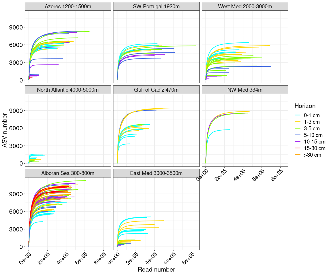
Figure S2: Taxonomic composition and alpha-diversity by location and horizon
general_taxo <- normal_by_sample_nb(ps = ps_sed_rel, X = "Horizon", facet = TRUE, Y = "Location_depth")
## phyloseq-class experiment-level object
## otu_table()   OTU Table:         [ 239314 taxa and 210 samples ]
## sample_data() Sample Data:       [ 210 samples by 28 sample variables ]
## tax_table()   Taxonomy Table:    [ 239314 taxa by 15 taxonomic ranks ]
general_taxo_phy <- tax_glom(general_taxo, taxrank=rank_names(general_taxo)[2], NArm=FALSE)

general_taxo_phy@sam_data$Location_depth <- factor(general_taxo_phy@sam_data$Location_depth,
                                                   levels = c("Azores 1200-1500m", "SW Portugal 1920m", "West Med 2000-3000m",
                                                              "North Atlantic 4000-5000m", "Gulf of Cadiz 470m", "NW Med 334m",
                                                              "Alboran Sea 300-800m", "East Med 3000-3500m"))

f2_2 <- plot_bar(general_taxo_phy, x = "Horizon", fill = "Phylum") +
  facet_wrap(~Location_depth) +
  scale_colour_manual(values=scale_taxon, na.value = "grey") +
  scale_fill_manual(values=scale_taxon, na.value = "grey") +
  geom_bar(aes(color= Phylum, fill= Phylum), stat = "identity", position = "stack", width = 0.75 )+
  theme_bw() +
  theme(axis.text.x= element_text(size=14,angle = 45, hjust = 1),
          axis.text.y = element_text(size = 16),
          axis.title.y = element_text(size = 16),
          axis.title.x = element_blank(),
          legend.title = element_text(size = 16),
          legend.text = element_text(size = 13),
          strip.text.x = element_text(size = 14)) +
  scale_x_discrete(labels = c("0_1"="0-1 cm", "1_3"="1-3 cm", "3_5"="3-5 cm", "5_10"="5-10 cm",
                              "10_15"="10-15 cm", "15_30"="15-30 cm", "30+"=">30 cm"))
# Ideally, Alboran and East Med should be moved to the right of the plot
f2_2
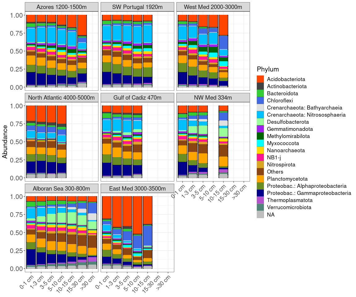
shannon <- estimate_richness(ps_sed, measures = "Shannon")

alpha_df <- data.frame(ps_sed@sam_data)
alpha_df$Alpha_div <- shannon$Shannon
alpha_df$Location_depth <- factor(alpha_df$Location_depth,
                                  levels = c("Azores 1200-1500m", "SW Portugal 1920m", "West Med 2000-3000m",
                                             "North Atlantic 4000-5000m", "Gulf of Cadiz 470m", "NW Med 334m",
                                             "Alboran Sea 300-800m", "East Med 3000-3500m"))

# Alpha diversity by location and horizon
alpha <- ggplot(alpha_df, aes(x = Horizon, y = Alpha_div)) +
  facet_wrap(~Location_depth) +
  geom_violin() + geom_boxplot(width=0.1,color="black") +
  theme_bw() +
  theme(axis.title.x=element_blank(),
        axis.text.x=element_text(size = 14, angle = 45, hjust = 1),
        axis.text.y = element_text(face="plain",size=16),
        axis.title.y = element_text(size=16),
        legend.text = element_text(size=13),
        legend.title = element_text(size=16),
        strip.text.x = element_text(size = 14))+
  scale_x_discrete(labels = c("0_1"="0-1 cm", "1_3"="1-3 cm", "3_5"="3-5 cm", "5_10"="5-10 cm",
                              "10_15"="10-15 cm", "15_30"="15-30 cm", "30+"=">30 cm")) +
  ylab("Alpha diversity - Shannon index")
alpha
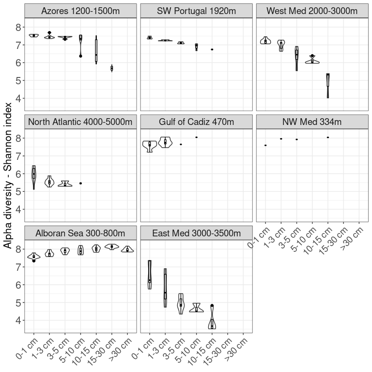
alpha_df[alpha_df$Location_depth == "North Atlantic 4000-5000m" | alpha_df$Location_depth == "East Med 3000-3500m", "Category"] <- "Lower_alpha"
alpha_df[is.na(alpha_df$Category), "Category"] <- "Higher_alpha"

kruskal.test(Alpha_div ~ Category, data = alpha_df)
##
##  Kruskal-Wallis rank sum test
##
## data:  Alpha_div by Category
## Kruskal-Wallis chi-squared = 90.046, df = 1, p-value < 2.2e-16
#pairwise.wilcox.test(alpha_df$Alpha_div, alpha_df$Category, p.adjust.method = "BH")
Figure S3: Taxonomy of biomarkers
Taxonomy of subsurface biomarkers
ps_subsurface <- subset_samples(ps_alboran, Horizon_category == "Subsurface")
ps_subsurface <- prune_taxa(taxa_sums(ps_subsurface)>0, ps_subsurface)

# overall subsurface
ps_biomarker_subsurface_overall <- prune_taxa(taxa = row.names(overall_subsurface_taxa), ps_subsurface)
ps_biomarker_subsurface_overall <- prune_samples(sample_sums(ps_biomarker_subsurface_overall)>0, ps_biomarker_subsurface_overall)
ps_biomarker_subsurface_overall
## phyloseq-class experiment-level object
## otu_table()   OTU Table:         [ 3427 taxa and 29 samples ]
## sample_data() Sample Data:       [ 29 samples by 30 sample variables ]
## tax_table()   Taxonomy Table:    [ 3427 taxa by 15 taxonomic ranks ]
df_overall_subsurface <- data.frame(ps_biomarker_subsurface_overall@tax_table[,c(1:6)])
df_overall_subsurface$Sequence <- rownames(df_overall_subsurface)
rownames(df_overall_subsurface) <- NULL
df_overall_subsurface$Relabund <- taxa_sums(ps_biomarker_subsurface_overall) / sum(sample_sums(ps_subsurface)) * 100
df_overall_subsurface <- setorder(df_overall_subsurface, -Relabund)
df_overall_subsurface_short <- df_overall_subsurface[c(1:50),]
df_overall_subsurface_short$ASV <- c(1:nrow(df_overall_subsurface_short))
df_overall_subsurface_short$ASV <- factor(df_overall_subsurface_short$ASV, levels =
                                            df_overall_subsurface_short$ASV[order(df_overall_subsurface_short$Relabund)]) # order by relative abundance

df_overall_subsurface_short$Site <- "Overall"
df_overall_subsurface_short$Label <- paste(df_overall_subsurface_short$Family, df_overall_subsurface_short$Shared)
df_overall_subsurface_short$Label <- gsub("NA" , "", df_overall_subsurface_short$Label)

gg <- ggplot(df_overall_subsurface_short, aes(x=ASV, y=Relabund, fill=Phylum)) +
  geom_bar(stat="identity") +
  facet_grid(~Site) +
  scale_y_continuous("Percent abundance of total community") +
  coord_flip()+
  scale_colour_manual(values=scale_55, na.value = "grey") +
  scale_fill_manual(values=scale_55, na.value = "grey") +
  geom_text(aes(label=Label), hjust="left", size=3)+
  theme_bw()+
  theme(axis.text.y = element_blank(), axis.ticks.y = element_blank(),
        plot.title = element_text(hjust = -0.05, size = 16, margin = margin(t = -5, b = 1)),
        strip.text = element_text(size = 12))
gg
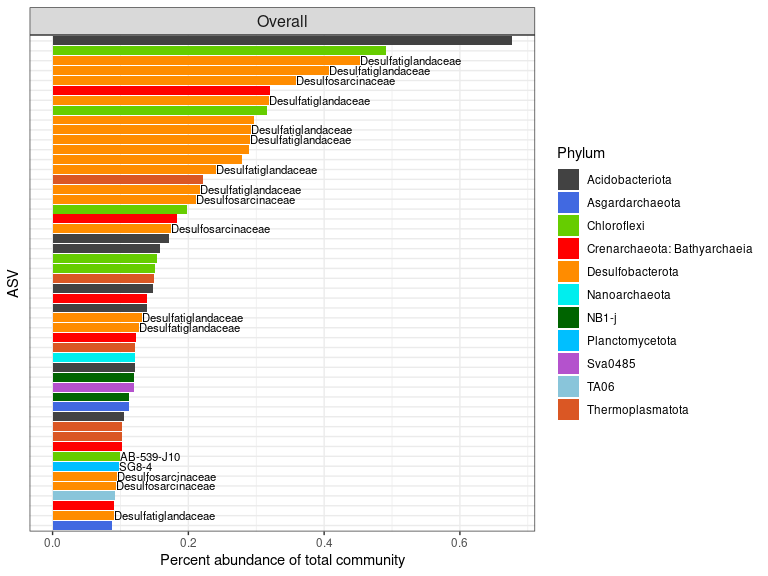
Taxonomy of site biomarkers
# site 215
ps_biomarker_site_215 <- prune_taxa(taxa_names(ps_215_surface) %in% row.names(biomarker_215), ps_215_surface)
df_site_215 <- data.frame(ps_biomarker_site_215@tax_table[,c(1:6)])
df_site_215$Sequence <- rownames(df_site_215)
rownames(df_site_215) <- NULL
df_site_215$Relabund <- taxa_sums(ps_biomarker_site_215) / sum(sample_sums(ps_215_surface)) * 100
df_site_215 <- setorder(df_site_215, -Relabund)
df_site_215_short <- df_site_215
df_site_215_short$ASV <- c(1:nrow(df_site_215_short))
df_site_215_short$ASV <- factor(df_site_215_short$ASV, levels = df_site_215_short$ASV[order(df_site_215_short$Relabund)]) # order by relative abundance

# site 201
ps_biomarker_site_201 <- prune_taxa(taxa_names(ps_201_surface) %in% row.names(biomarker_201), ps_201_surface)
df_site_201 <- data.frame(ps_biomarker_site_201@tax_table[,c(1:6)])
df_site_201$Sequence <- rownames(df_site_201)
rownames(df_site_201) <- NULL
df_site_201$Relabund <- taxa_sums(ps_biomarker_site_201) / sum(sample_sums(ps_201_surface)) * 100
df_site_201 <- setorder(df_site_201, -Relabund)
df_site_201_short <- df_site_201
df_site_201_short$ASV <- c(1:nrow(df_site_201_short))
df_site_201_short$ASV <- factor(df_site_201_short$ASV, levels = df_site_201_short$ASV[order(df_site_201_short$Relabund)]) # order by relative abundance

# site 179
ps_biomarker_site_179 <- prune_taxa(taxa_names(ps_179_surface) %in% row.names(biomarker_179), ps_179_surface)
df_site_179 <- data.frame(ps_biomarker_site_179@tax_table[,c(1:6)])
df_site_179$Sequence <- rownames(df_site_179)
rownames(df_site_179) <- NULL
df_site_179$Relabund <- taxa_sums(ps_biomarker_site_179) / sum(sample_sums(ps_179_surface)) * 100
df_site_179 <- setorder(df_site_179, -Relabund)
df_site_179_short <- df_site_179[c(1:50),]
df_site_179_short$ASV <- c(1:nrow(df_site_179_short))
df_site_179_short$ASV <- factor(df_site_179_short$ASV, levels = df_site_179_short$ASV[order(df_site_179_short$Relabund)]) # order by relative abundance

length(intersect(intersect(df_site_179_short$Sequence, df_site_215_short$Sequence), df_site_201_short$Sequence))
## [1] 0
# no intersect
df_site_179_short$Site <- "MDW_Site179"
df_site_215_short$Site <- "MDW_Site215"
df_site_201_short$Site <- "MDW_Site201"

df_site_short <- rbind(df_site_179_short, df_site_215_short, df_site_201_short)

gg <- ggplot(df_site_short, aes(x=ASV, y=Relabund, fill=Phylum)) +
  geom_bar(stat="identity") +
  facet_grid(~Site) +
  scale_y_continuous("Percent abundance of total community") +
  coord_flip()+
  scale_colour_manual(values=scale_55, na.value = "grey") +
  scale_fill_manual(values=scale_55, na.value = "grey") +
  geom_text(aes(label=Family), hjust="left", size=3)+
  theme_bw()+
  theme(axis.text.y = element_blank(), axis.ticks.y = element_blank(),
        plot.title = element_text(hjust = -0.05, size = 16, margin = margin(t = -5, b = 1)),
        strip.text = element_text(size = 12), legend.position = "bottom", legend.direction="vertical")
gg
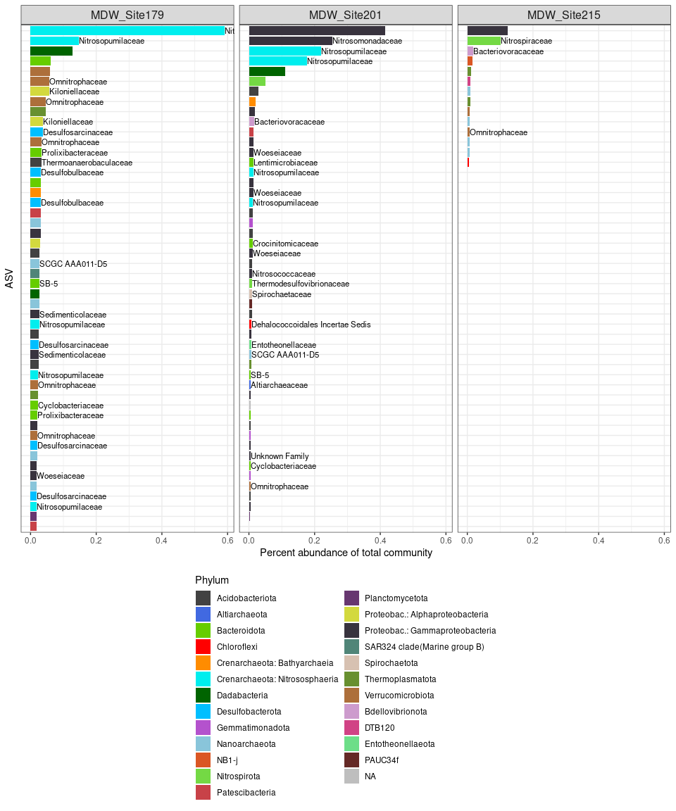
Figure S4: Global variation partitioning
# environmental data is scaled and centered during varpart
ps_sed_varpart <- prune_samples(intersect(sample_names(ps_sed_norm), rownames(env_data)), ps_sed_norm)
ps_sed_varpart <- prune_taxa(taxa_sums(ps_sed_varpart) > 0, ps_sed_varpart)

geo_df_short <- as.data.frame(as.matrix(ps_sed_varpart@sam_data[,c("Longitude","Latitude")]))
geo_df_short$Longitude <- as.numeric(as.character(geo_df_short$Longitude))
geo_df_short$Latitude <- as.numeric(as.character(geo_df_short$Latitude))
geo_df_short$X2 <- geo_df_short$Latitude^2

bc_dist <- vegdist(t(ps_sed_varpart@otu_table), method = "bray")

var.part1 <- varpart(bc_dist, geo_df_short, env_data)
showvarparts(2, labels=as.character(round(var.part1$part$indfract$Adj.R.square, 3)*100),
             bg=c("red","green"), Xnames = c("Spatial","Environmental"))
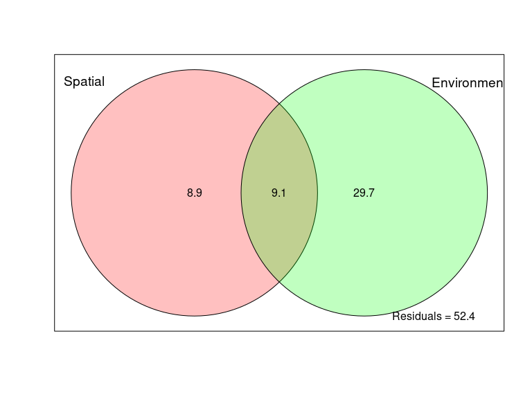
# testing significance
rda.all <- dbrda(bc_dist ~ Longitude+Latitude+X2+Depth+Temperature+Horizon+Shore_dist+Water_mean+MO_mean+Dv43_mean+dv_span_mean, data = c(geo_df_short, env_data))
anova(rda.all)
## Permutation test for dbrda under reduced model
## Permutation: free
## Number of permutations: 999
##
## Model: dbrda(formula = bc_dist ~ Longitude + Latitude + X2 + Depth + Temperature + Horizon + Shore_dist + Water_mean + MO_mean + Dv43_mean + dv_span_mean, data = c(geo_df_short, env_data))
##           Df SumOfSqs      F Pr(>F)
## Model     11   36.966 16.054  0.001 ***
## Residual 171   35.795
## ---
## Signif. codes:  0 '***' 0.001 '**' 0.01 '*' 0.05 '.' 0.1 ' ' 1
rda.space <- dbrda (bc_dist ~ Longitude+Latitude+X2, data = geo_df_short)
anova(rda.space)
## Permutation test for dbrda under reduced model
## Permutation: free
## Number of permutations: 999
##
## Model: dbrda(formula = bc_dist ~ Longitude + Latitude + X2, data = geo_df_short)
##           Df SumOfSqs      F Pr(>F)
## Model      3   14.014 14.233  0.001 ***
## Residual 179   58.747
## ---
## Signif. codes:  0 '***' 0.001 '**' 0.01 '*' 0.05 '.' 0.1 ' ' 1
rda.env <- dbrda (bc_dist ~ Depth+Temperature+Horizon+Shore_dist+Water_mean+MO_mean+Dv43_mean+dv_span_mean, data = env_data)
anova(rda.env)
## Permutation test for dbrda under reduced model
## Permutation: free
## Number of permutations: 999
##
## Model: dbrda(formula = bc_dist ~ Depth + Temperature + Horizon + Shore_dist + Water_mean + MO_mean + Dv43_mean + dv_span_mean, data = env_data)
##           Df SumOfSqs      F Pr(>F)
## Model      8   30.181 15.416  0.001 ***
## Residual 174   42.580
## ---
## Signif. codes:  0 '***' 0.001 '**' 0.01 '*' 0.05 '.' 0.1 ' ' 1
rda.space.env <- dbrda (bc_dist ~ Longitude+Latitude+X2 + Condition(Depth+Temperature+Horizon+Shore_dist+Water_mean+MO_mean+Dv43_mean+dv_span_mean),
                        data = c(geo_df_short, env_data))
anova(rda.space.env)
## Permutation test for dbrda under reduced model
## Permutation: free
## Number of permutations: 999
##
## Model: dbrda(formula = bc_dist ~ Longitude + Latitude + X2 + Condition(Depth + Temperature + Horizon + Shore_dist + Water_mean + MO_mean + Dv43_mean + dv_span_mean), data = c(geo_df_short, env_data))
##           Df SumOfSqs      F Pr(>F)
## Model      3    6.785 10.804  0.001 ***
## Residual 171   35.795
## ---
## Signif. codes:  0 '***' 0.001 '**' 0.01 '*' 0.05 '.' 0.1 ' ' 1
rda.env.space <- dbrda (bc_dist ~ Depth+Temperature+Horizon+Shore_dist+Water_mean+MO_mean+Dv43_mean+dv_span_mean + Condition(Longitude+Latitude+X2),
                        data = c(geo_df_short, env_data))
anova(rda.env.space)
## Permutation test for dbrda under reduced model
## Permutation: free
## Number of permutations: 999
##
## Model: dbrda(formula = bc_dist ~ Depth + Temperature + Horizon + Shore_dist + Water_mean + MO_mean + Dv43_mean + dv_span_mean + Condition(Longitude + Latitude + X2), data = c(geo_df_short, env_data))
##           Df SumOfSqs      F Pr(>F)
## Model      8   22.952 13.706  0.001 ***
## Residual 171   35.795
## ---
## Signif. codes:  0 '***' 0.001 '**' 0.01 '*' 0.05 '.' 0.1 ' ' 1
var.part2 <- varpart(bc_dist, geo_df_short,
                     env_data[, "Depth"],
                    env_data[, "Temperature"],
                    env_data[, "Horizon"])
showvarparts(4,labels=as.character(round(var.part2$part$indfract$Adj.R.square, 3)*100),
             bg=c("red","blue","green", "cyan"), Xnames = c("Spatial", "Depth", "Temperature", "Horizon"))
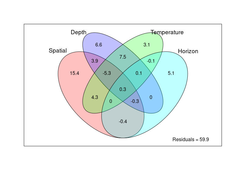
# testing significance
rda.all <- dbrda(bc_dist ~ Longitude+Latitude+X2+Depth+Temperature+Horizon, data = c(geo_df_short, env_data))
anova(rda.all)
## Permutation test for dbrda under reduced model
## Permutation: free
## Number of permutations: 999
##
## Model: dbrda(formula = bc_dist ~ Longitude + Latitude + X2 + Depth + Temperature + Horizon, data = c(geo_df_short, env_data))
##           Df SumOfSqs      F Pr(>F)
## Model      6   30.634 21.331  0.001 ***
## Residual 176   42.126
## ---
## Signif. codes:  0 '***' 0.001 '**' 0.01 '*' 0.05 '.' 0.1 ' ' 1
rda.space <- dbrda (bc_dist ~ Longitude+Latitude+X2, data = geo_df_short)
anova(rda.space)
## Permutation test for dbrda under reduced model
## Permutation: free
## Number of permutations: 999
##
## Model: dbrda(formula = bc_dist ~ Longitude + Latitude + X2, data = geo_df_short)
##           Df SumOfSqs      F Pr(>F)
## Model      3   14.014 14.233  0.001 ***
## Residual 179   58.747
## ---
## Signif. codes:  0 '***' 0.001 '**' 0.01 '*' 0.05 '.' 0.1 ' ' 1
rda.env <- dbrda (bc_dist ~ Depth+Temperature+Horizon, data = env_data)
anova(rda.env)
## Permutation test for dbrda under reduced model
## Permutation: free
## Number of permutations: 999
##
## Model: dbrda(formula = bc_dist ~ Depth + Temperature + Horizon, data = env_data)
##           Df SumOfSqs      F Pr(>F)
## Model      3   18.884 20.914  0.001 ***
## Residual 179   53.876
## ---
## Signif. codes:  0 '***' 0.001 '**' 0.01 '*' 0.05 '.' 0.1 ' ' 1
rda.space.env <- dbrda (bc_dist ~ Longitude+Latitude+X2 + Condition(Depth+Temperature+Horizon),
                        data = c(geo_df_short, env_data))
anova(rda.space.env)
## Permutation test for dbrda under reduced model
## Permutation: free
## Number of permutations: 999
##
## Model: dbrda(formula = bc_dist ~ Longitude + Latitude + X2 + Condition(Depth + Temperature + Horizon), data = c(geo_df_short, env_data))
##           Df SumOfSqs      F Pr(>F)
## Model      3   11.750 16.363  0.001 ***
## Residual 176   42.126
## ---
## Signif. codes:  0 '***' 0.001 '**' 0.01 '*' 0.05 '.' 0.1 ' ' 1
rda.env.space <- dbrda (bc_dist ~ Depth+Temperature+Horizon + Condition(Longitude+Latitude+X2),
                        data = c(geo_df_short, env_data))
anova(rda.env.space)
## Permutation test for dbrda under reduced model
## Permutation: free
## Number of permutations: 999
##
## Model: dbrda(formula = bc_dist ~ Depth + Temperature + Horizon + Condition(Longitude + Latitude + X2), data = c(geo_df_short, env_data))
##           Df SumOfSqs      F Pr(>F)
## Model      3   16.621 23.146  0.001 ***
## Residual 176   42.126
## ---
## Signif. codes:  0 '***' 0.001 '**' 0.01 '*' 0.05 '.' 0.1 ' ' 1
var.part2 <- varpart(bc_dist, env_data[, "Depth"],
                    env_data[, "Temperature"],
                    env_data[, "Horizon"],
                    env_data[, "Water_mean"] + env_data[, "MO_mean"] + env_data[, "Dv43_mean"] + env_data[, "dv_span_mean"])
showvarparts(4,labels=as.character(round(var.part2$part$indfract$Adj.R.square, 3)*100),
             bg=c("blue","green", "cyan", "gold"), Xnames = c("Depth", "Temperature", "Horizon", "Sediment composition"))
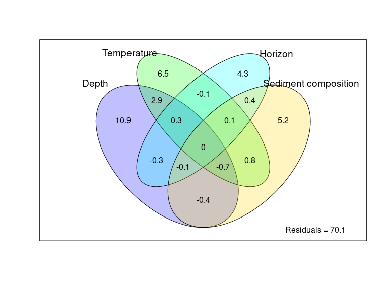
# testing significance
rda.all <- dbrda(bc_dist ~ Depth+Temperature+Horizon+Water_mean+MO_mean+Dv43_mean+dv_span_mean, data = env_data)
anova(rda.all)
## Permutation test for dbrda under reduced model
## Permutation: free
## Number of permutations: 999
##
## Model: dbrda(formula = bc_dist ~ Depth + Temperature + Horizon + Water_mean + MO_mean + Dv43_mean + dv_span_mean, data = env_data)
##           Df SumOfSqs      F Pr(>F)
## Model      7   27.171 14.899  0.001 ***
## Residual 175   45.590
## ---
## Signif. codes:  0 '***' 0.001 '**' 0.01 '*' 0.05 '.' 0.1 ' ' 1
rda.space <- dbrda (bc_dist ~ Depth, data = env_data)
anova(rda.space)
## Permutation test for dbrda under reduced model
## Permutation: free
## Number of permutations: 999
##
## Model: dbrda(formula = bc_dist ~ Depth, data = env_data)
##           Df SumOfSqs      F Pr(>F)
## Model      1    9.554 27.358  0.001 ***
## Residual 181   63.207
## ---
## Signif. codes:  0 '***' 0.001 '**' 0.01 '*' 0.05 '.' 0.1 ' ' 1
rda.env <- dbrda (bc_dist ~ Temperature, data = env_data)
anova(rda.env)
## Permutation test for dbrda under reduced model
## Permutation: free
## Number of permutations: 999
##
## Model: dbrda(formula = bc_dist ~ Temperature, data = env_data)
##           Df SumOfSqs      F Pr(>F)
## Model      1    7.514 20.844  0.001 ***
## Residual 181   65.247
## ---
## Signif. codes:  0 '***' 0.001 '**' 0.01 '*' 0.05 '.' 0.1 ' ' 1
rda.sed <- dbrda (bc_dist ~ Water_mean+MO_mean+Dv43_mean+dv_span_mean, data = env_data)
anova(rda.sed)
## Permutation test for dbrda under reduced model
## Permutation: free
## Number of permutations: 999
##
## Model: dbrda(formula = bc_dist ~ Water_mean + MO_mean + Dv43_mean + dv_span_mean, data = env_data)
##           Df SumOfSqs      F Pr(>F)
## Model      4   11.275 8.1606  0.001 ***
## Residual 178   61.485
## ---
## Signif. codes:  0 '***' 0.001 '**' 0.01 '*' 0.05 '.' 0.1 ' ' 1
var.part3 <- varpart(bc_dist, env_data[, "Water_mean"],
                     env_data[, "MO_mean"],
                     env_data[, "Dv43_mean"],
                     env_data[, "dv_span_mean"])
showvarparts(4,labels=as.character(round(var.part3$part$indfract$Adj.R.square, 3)*100),
             bg=c("blue","red","green", "cyan"), Xnames = c("Humidity level", "OM content", "Mean granulometry", "Size heterogeneity"))
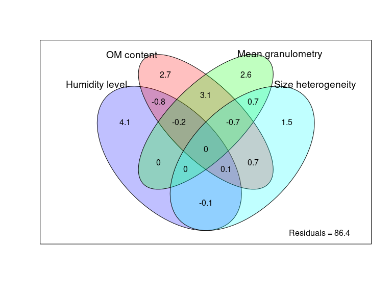
Figure S5: Sedimentary composition by depth zone
meta_df <- data.frame(ps_sed_norm@sam_data)
meta_df$Water_mean <- as.numeric(as.character(meta_df$Water_mean))
meta_df$MO_mean <- as.numeric(as.character(meta_df$MO_mean))
meta_df$Dv43_mean <- as.numeric(as.character(meta_df$Dv43_mean))

# boxplot
q_water <- ggplot(meta_df, aes(x = Zone, y = Water_mean)) +
  geom_boxplot(width=0.5,color="black") +
  ggtitle("Humidity level") +
  theme_bw() + theme(axis.title.x=element_blank(),
        axis.text.x=element_blank(),
        axis.text.y = element_text(face="plain", size=15),
        axis.title.y = element_blank(),
        plot.title = element_text(size = 16, hjust = 0.5))

q_MO <- ggplot(meta_df, aes(x = Zone, y = MO_mean)) +
  geom_boxplot(width=0.5,color="black") +
  ggtitle("Organic matter content") +
  theme_bw() + theme(axis.title.x=element_blank(),
        axis.text.x=element_blank(),
        axis.text.y = element_text(face="plain", size=15),
        axis.title.y = element_blank(),
        plot.title = element_text(size = 16, hjust = 0.5))

q_granulo <- ggplot(meta_df, aes(x = Zone, y = Dv43_mean)) +
  geom_boxplot(width=0.5,color="black") +
  ggtitle("Mean granulometry") +
  theme_bw() + theme(axis.title.x=element_blank(),
        axis.text.x = element_text(angle=45, size = 15, vjust=1, hjust = 1),
        axis.text.y = element_text(face="plain", size=15),
        axis.title.y = element_blank(),
        plot.title = element_text(size = 16, hjust = 0.5)) +
  scale_x_discrete(labels = c("Upper bathyal", "Lower bathyal", "Abyssal"))

q_span <- ggplot(meta_df, aes(x = Zone, y = dv_span_mean)) +
  geom_boxplot(width=0.5,color="black") +
  ggtitle("Particle size (heterogeneity)") +
  theme_bw() + theme(axis.title.x=element_blank(),
        axis.text.x=element_text(angle=45, size = 15, vjust=1, hjust = 1),
        axis.text.y = element_text(face="plain", size=15),
        axis.title.y = element_blank(),
        plot.title = element_text(size = 16, hjust = 0.5)) +
  scale_x_discrete(labels = c("Upper bathyal zone", "Lower bathyal zone", "Abyssal zone"))

q_water + q_MO + q_granulo + q_span
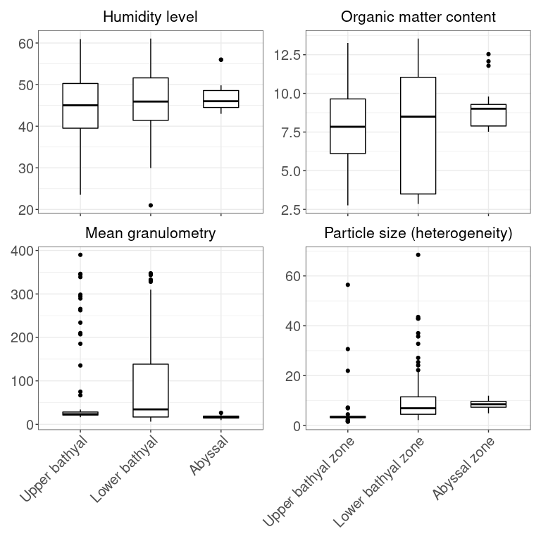
# Water content
kruskal.test(Water_mean ~ Zone, data = meta_df)
##
##  Kruskal-Wallis rank sum test
##
## data:  Water_mean by Zone
## Kruskal-Wallis chi-squared = 2.4753, df = 2, p-value = 0.2901
# no significant difference

# OM content
kruskal.test(MO_mean ~ Zone, data = meta_df)
##
##  Kruskal-Wallis rank sum test
##
## data:  MO_mean by Zone
## Kruskal-Wallis chi-squared = 6.5121, df = 2, p-value = 0.03854
pairwise.wilcox.test(meta_df$MO_mean, meta_df$Zone, p.adjust.method = "BH")
##
##  Pairwise comparisons using Wilcoxon rank sum test
##
## data:  meta_df$MO_mean and meta_df$Zone
##
##                            Upper bathyal (300-800m) Lower bathyal (1200-3500m)
## Lower bathyal (1200-3500m) 0.055                    -
## Abyssal (4000m+)           0.055                    0.507
##
## P value adjustment method: BH
# not significant

# Mean granulo
kruskal.test(Dv43_mean ~ Zone, data = meta_df)
##
##  Kruskal-Wallis rank sum test
##
## data:  Dv43_mean by Zone
## Kruskal-Wallis chi-squared = 21.534, df = 2, p-value = 2.109e-05
pairwise.wilcox.test(meta_df$Dv43_mean, meta_df$Zone, p.adjust.method = "BH")
##
##  Pairwise comparisons using Wilcoxon rank sum test
##
## data:  meta_df$Dv43_mean and meta_df$Zone
##
##                            Upper bathyal (300-800m) Lower bathyal (1200-3500m)
## Lower bathyal (1200-3500m) 0.71450                  -
## Abyssal (4000m+)           2e-07                    0.00037
##
## P value adjustment method: BH
# significant difference between upper bathyal/abyssal and lower bathyal/abyssal

# heterogeneity (granulo)
kruskal.test(dv_span_mean ~ Zone, data = meta_df)
##
##  Kruskal-Wallis rank sum test
##
## data:  dv_span_mean by Zone
## Kruskal-Wallis chi-squared = 65.506, df = 2, p-value = 5.963e-15
pairwise.wilcox.test(meta_df$dv_span_mean, meta_df$Zone, p.adjust.method = "BH")
##
## Pairwise comparisons using Wilcoxon rank sum test
##
## data: meta_df$dv_span_mean and meta_df$Zone
##
## Upper bathyal (300-800m) Lower bathyal (1200-3500m)
## Lower bathyal (1200-3500m) 1.2e-12 -
## Abyssal (4000m+) 2.3e-09 0.2
##
## P value adjustment method: BH
# significant difference between upper bathyal/lower bathyal and upper bathyal/abyssal
Additional analyses (mentionned in paper)
Depth distinction between upper and lower bathyal zones
Focusing on geographically close sites of the upper bathyal zone: Alboran, Gibraltar, NW Med Comparison with geographically close sites of the lower bathyal zone: SW Portugal and West Med Restricting to the top 3 horizons (up to 5 cmbsf) since community composition diverges with horizon depth. 79 samples and 129,986 taxa
ps_comp <- subset_samples(ps_sed_norm, Cruise != "AMIGO1")
ps_comp <- subset_samples(ps_comp, Location != "Azores (Formigas seamount)")
ps_comp <- subset_samples(ps_comp, Site != "PCT_I" & Site != "PCT_T")
ps_comp <- subset_samples(ps_comp, Horizon == "0_1" | Horizon == "1_3" | Horizon == "3_5")
ps_comp <- prune_taxa(taxa_sums(ps_comp) > 0, ps_comp)
library(UpSetR)
# Number of ASVs shared between depth ranges
graph <- graph_for_upset(ps_comp, "Zone")
### production du graph upset
upset(fromList(graph), sets = c("Upper bathyal (300-800m)", "Lower bathyal (1200-3500m)"),
keep.order = TRUE,
order.by = "freq")
grid.text("ASVs shared between upper and lower bathyal zones", x = 0.65, y=0.95, gp=gpar(fontsize=20))
# based on location_depth range
ps_comp@sam_data$Loc_depth <- ps_comp@sam_data$Depth
ps_comp@sam_data$Loc_depth <- gsub("334", "NW_med_upper", ps_comp@sam_data$Loc_depth)
ps_comp@sam_data$Loc_depth <- gsub("729|381|554|470", "Transition_upper", ps_comp@sam_data$Loc_depth)
ps_comp@sam_data$Loc_depth <- gsub("1920|2800", "Transition_lower", ps_comp@sam_data$Loc_depth)
ps_comp@sam_data$Loc_depth <- gsub("2415|2417|2418|2490", "NW_med_lower", ps_comp@sam_data$Loc_depth)
graph <- graph_for_upset(ps_comp, "Loc_depth")
upset(fromList(graph), sets = c("NW_med_upper", "NW_med_lower", "Transition_upper", "Transition_lower"),
keep.order = TRUE,
order.by = "freq")
grid.text("ASVs shared between upper and lower bathyal zones", x = 0.65, y=0.95, gp=gpar(fontsize=20))
# relative abundance
intersect_percent <- data.table("Community" = c("NW_med_upper", "Transition_upper"),
"Site_specific" = c(0,0),
"Shared_upper" = c(0,0),
"Shared_adjacent_lower" = c(0,0),
"Shared_all" = c(0,0))
ps_med_meso <- subset_samples(ps_comp, Loc_depth == "NW_med_upper")
ps_trans_meso <- subset_samples(ps_comp, Loc_depth == "Transition_upper")
intersect_percent$Site_specific[1] <- sum(sample_sums(
prune_taxa(setdiff(setdiff(graph$NW_med_upper, graph$NW_med_lower), graph$Transition_upper), ps_med_meso))) /
sum(sample_sums(ps_med_meso)) * 100
intersect_percent$Site_specific[2] <- sum(sample_sums(
prune_taxa(setdiff(setdiff(graph$Transition_upper, graph$Transition_lower), graph$NW_med_upper), ps_trans_meso))) /
sum(sample_sums(ps_trans_meso)) * 100
intersect_percent$Shared_upper[1] <- sum(sample_sums(
prune_taxa(setdiff(intersect(graph$NW_med_upper, graph$Transition_upper), graph$NW_med_lower), ps_med_meso))) /
sum(sample_sums(ps_med_meso)) * 100
intersect_percent$Shared_adjacent_lower[1] <- sum(sample_sums(
prune_taxa(setdiff(intersect(graph$NW_med_upper, graph$NW_med_lower), graph$Transition_upper), ps_med_meso))) /
sum(sample_sums(ps_med_meso)) * 100
intersect_percent$Shared_all[1] <- sum(sample_sums(
prune_taxa(Reduce(intersect, list(graph$NW_med_upper, graph$NW_med_lower, graph$Transition_upper)), ps_med_meso))) /
sum(sample_sums(ps_med_meso)) * 100
intersect_percent$Shared_upper[2] <- sum(sample_sums(
prune_taxa(setdiff(intersect(graph$NW_med_upper, graph$Transition_upper), graph$Transition_lower), ps_trans_meso))) /
sum(sample_sums(ps_trans_meso)) * 100
intersect_percent$Shared_adjacent_lower[2] <- sum(sample_sums(
prune_taxa(setdiff(intersect(graph$Transition_upper, graph$Transition_lower), graph$NW_med_upper), ps_trans_meso))) /
sum(sample_sums(ps_trans_meso)) * 100
intersect_percent$Shared_all[2] <- sum(sample_sums(
prune_taxa(Reduce(intersect, list(graph$NW_med_upper, graph$Transition_lower, graph$Transition_upper)), ps_trans_meso))) /
sum(sample_sums(ps_trans_meso)) * 100
melt_intersect <- melt(intersect_percent, id.vars = c("Community"))
gg <- ggplot(melt_intersect, aes(x = Community, y = value, fill = variable)) +
geom_bar(stat = "identity", position = "stack") +
theme(axis.text.x = element_text(size = 12, angle = 0),
axis.title.x = element_blank(),
axis.text.y = element_text(size = 12),
axis.title.y = element_text(size = 14),
legend.position="right",
legend.title = element_blank(),
legend.text = element_text(size = 14),
plot.title = element_text(size = 18)) +
ggtitle("Composition of communities in terms of shared ASVs")
gg
Local scale: shared vs specific community (quant and qual) and patchiness of rare ASVs
# Number of ASVs shared between depth ranges
graph <- graph_for_upset(ps_alboran, "Site")
### production du graph upset
upset(fromList(graph), sets = c("MDW_ST215", "MDW_ST201", "MDW_ST179"),
keep.order = TRUE,
order.by = "freq")
grid.text("ASVs shared between Alboran sites", x = 0.65, y=0.95, gp=gpar(fontsize=20))
# relative abundance
intersect_percent <- data.table("Site" = c("MDW_ST201", "MDW_ST215", "MDW_ST179"),
"Site_specific" = c(0,0,0),
"Shared_adj_1" = c(0,0,0),
"Shared_adj_2" = c(0,0,0),
"Shared_all" = c(0,0,0))
# site-specific
intersect_percent$Site_specific[1] <- sum(sample_sums(
prune_taxa(setdiff(setdiff(graph$MDW_ST201, graph$MDW_ST215), graph$MDW_ST179), ps_201))) /
sum(sample_sums(ps_201)) * 100
intersect_percent$Site_specific[2] <- sum(sample_sums(
prune_taxa(setdiff(setdiff(graph$MDW_ST215, graph$MDW_ST201), graph$MDW_ST179), ps_215))) /
sum(sample_sums(ps_215)) * 100
intersect_percent$Site_specific[3] <- sum(sample_sums(
prune_taxa(setdiff(setdiff(graph$MDW_ST179, graph$MDW_ST201), graph$MDW_ST215), ps_179))) /
sum(sample_sums(ps_179)) * 100
# site 201
intersect_percent$Shared_adj_1[1] <- sum(sample_sums(
prune_taxa(setdiff(intersect(graph$MDW_ST201, graph$MDW_ST215), graph$MDW_ST179), ps_201))) /
sum(sample_sums(ps_201)) * 100
intersect_percent$Shared_adj_2[1] <- sum(sample_sums(
prune_taxa(setdiff(intersect(graph$MDW_ST201, graph$MDW_ST179), graph$MDW_ST215), ps_201))) /
sum(sample_sums(ps_201)) * 100
intersect_percent$Shared_all[1] <- sum(sample_sums(
prune_taxa(Reduce(intersect, list(graph$MDW_ST201, graph$MDW_ST215, graph$MDW_ST179)), ps_201))) /
sum(sample_sums(ps_201)) * 100
# site 215
intersect_percent$Shared_adj_1[2] <- sum(sample_sums(
prune_taxa(setdiff(intersect(graph$MDW_ST215, graph$MDW_ST201), graph$MDW_ST179), ps_215))) /
sum(sample_sums(ps_215)) * 100
intersect_percent$Shared_adj_2[2] <- sum(sample_sums(
prune_taxa(setdiff(intersect(graph$MDW_ST215, graph$MDW_ST179), graph$MDW_ST201), ps_215))) /
sum(sample_sums(ps_215)) * 100
intersect_percent$Shared_all[2] <- sum(sample_sums(
prune_taxa(Reduce(intersect, list(graph$MDW_ST215, graph$MDW_ST201, graph$MDW_ST179)), ps_215))) /
sum(sample_sums(ps_215)) * 100
# site 179
intersect_percent$Shared_adj_1[3] <- sum(sample_sums(
prune_taxa(setdiff(intersect(graph$MDW_ST179, graph$MDW_ST201), graph$MDW_ST215), ps_179))) /
sum(sample_sums(ps_179)) * 100
intersect_percent$Shared_adj_2[3] <- sum(sample_sums(
prune_taxa(setdiff(intersect(graph$MDW_ST179, graph$MDW_ST215), graph$MDW_ST201), ps_179))) /
sum(sample_sums(ps_179)) * 100
intersect_percent$Shared_all[3] <- sum(sample_sums(
prune_taxa(Reduce(intersect, list(graph$MDW_ST179, graph$MDW_ST201, graph$MDW_ST215)), ps_179))) /
sum(sample_sums(ps_179)) * 100
intersect_percent
## Site Site_specific Shared_adj_1 Shared_adj_2 Shared_all
## 1: MDW_ST201 6.980573 7.383085 2.305028 83.33131
## 2: MDW_ST215 4.258586 5.216709 4.706116 85.81859
## 3: MDW_ST179 9.532207 2.701864 7.289695 80.47623
melt_intersect <- melt(intersect_percent, id.vars = c("Site"))
gg <- ggplot(melt_intersect, aes(x = Site, y = value, fill = variable)) +
geom_bar(stat = "identity", position = "stack") +
theme(axis.text.x = element_text(size = 12, angle = 0),
axis.title.x = element_blank(),
axis.text.y = element_text(size = 12),
axis.title.y = element_text(size = 14),
legend.position="right",
legend.title = element_blank(),
legend.text = element_text(size = 14),
plot.title = element_text(size = 18)) +
ggtitle("Composition of communities in terms of shared ASVs")
gg
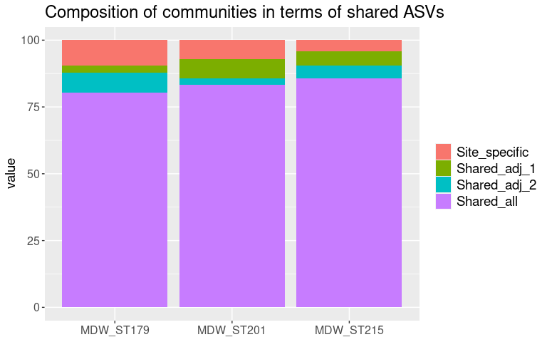
Looking at patchiness of ASVs between sites and between cores of the same site in Alboran
test <- transform_sample_counts(ps_alboran, function(x) (x/sum(x)*100))
df_asv <- data.frame(test@tax_table[,c(1:2)])
df_asv$percent <- signif((taxa_sums(test) / 65), 3)
df_asv <- df_asv[df_asv$percent<0.0007,]
# I keep as rare ASVs all below 0.0007, because this is the relative abundance that would exist if the community was evenly distributed
# There are 122,237 rare ASVs (out of 137,495), and the abundant ASVs represent 88% of the community.
rare_alboran <- prune_taxa(taxa_names(ps_alboran) %in% rownames(df_asv), ps_alboran)
# Bray-Curtis distance between communities
bc_dist <- vegdist(t(rare_alboran@otu_table), method = "bray")
# Bray-Curtis distance between communities as a function of geographical distance
bc_dist <- as.matrix(bc_dist)
df_distances <- melt(bc_dist, na.rm = TRUE)
colnames(df_distances) <- c("Sample1", "Sample2", "BC_dist")
df_distances <- df_distances[df_distances$Sample1 != df_distances$Sample2,]
data <- rare_alboran@sam_data[match(df_distances$Sample1, rownames(rare_alboran@sam_data)),]
df_distances$Sample1_horizon = data$True_horizon
df_distances$Sample1_site = data$Site
df_distances$Sample1_core = data$Core
data <- rare_alboran@sam_data[match(df_distances$Sample2, rownames(rare_alboran@sam_data)),]
df_distances$Sample2_horizon = data$True_horizon
df_distances$Sample2_site = data$Site
df_distances$Sample2_core = data$Core
df_distances <- df_distances[-grep("40_50", df_distances$Sample1_horizon),]
df_distances <- df_distances[-grep("40_50", df_distances$Sample2_horizon),]
Boxplots to check if Bray-Curtis dissimilarity is higher between sites than between cores of one site
df_by_horizon <- df_distances[df_distances$Sample1_horizon == df_distances$Sample2_horizon,]
dim(df_by_horizon)
## [1] 504 9
horizon <- ggplot(df_by_horizon, aes(x = Sample1_horizon, y = BC_dist, fill = Sample1_site)) +
facet_grid(Sample2_site~.) +
geom_boxplot(width=0.5,color="black") +
scale_y_continuous(name = "Bray-Curtis distance", breaks = c(0.2, 0.4, 0.6, 0.8)) +
theme_bw() + theme(axis.title.x=element_blank(),
axis.text.x=element_text(size = 15),
axis.text.y = element_text(face="plain",size=15),
axis.title.y = element_text(size=18),
strip.text.x = element_text(size = 20),
title = element_text(size = 18))
horizon
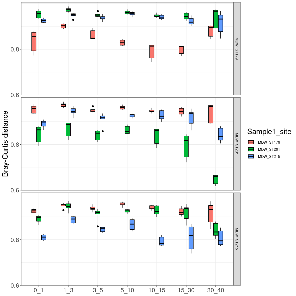
sessionInfo()
## R version 3.6.1 (2019-07-05)
## Platform: x86_64-pc-linux-gnu (64-bit)
## Running under: CentOS Linux 7 (Core)
##
## Matrix products: default
## BLAS/LAPACK: /home/usrlocal/OpenBLAS/lib/libopenblas_sandybridgep-r0.3.13.so
##
## Random number generation:
## RNG: Mersenne-Twister
## Normal: Inversion
## Sample: Rounding
##
## locale:
## [1] LC_CTYPE=fr_FR.UTF-8 LC_NUMERIC=C
## [3] LC_TIME=fr_FR.UTF-8 LC_COLLATE=fr_FR.UTF-8
## [5] LC_MONETARY=fr_FR.UTF-8 LC_MESSAGES=fr_FR.UTF-8
## [7] LC_PAPER=fr_FR.UTF-8 LC_NAME=C
## [9] LC_ADDRESS=C LC_TELEPHONE=C
## [11] LC_MEASUREMENT=fr_FR.UTF-8 LC_IDENTIFICATION=C
##
## attached base packages:
## [1] grid parallel stats4 stats graphics grDevices utils
## [8] datasets methods base
##
## other attached packages:
## [1] rmarkdown_2.6 plotrix_3.8-1
## [3] metagenomeSeq_1.26.3 glmnet_4.1-1
## [5] Matrix_1.2-17 limma_3.40.6
## [7] ggrepel_0.9.1 corrplot_0.84
## [9] Hmisc_4.3-0 Formula_1.2-4
## [11] survival_2.44-1.1 missMDA_1.18
## [13] factoextra_1.0.7 FactoMineR_2.4
## [15] maps_3.3.0 ggmap_3.0.0
## [17] enmSdm_0.5.3.2 dismo_1.3-3
## [19] raster_3.4-5 sp_1.4-5
## [21] gridExtra_2.3 speedyseq_0.1.2.9004
## [23] patchwork_1.1.1 simba_0.3-5
## [25] broom_0.7.3 ggpmisc_0.3.8
## [27] geosphere_1.5-10 tidyr_1.1.2
## [29] UpSetR_1.4.0 dplyr_1.0.3
## [31] DESeq2_1.24.0 SummarizedExperiment_1.14.1
## [33] DelayedArray_0.10.0 BiocParallel_1.18.1
## [35] matrixStats_0.58.0 Biobase_2.44.0
## [37] GenomicRanges_1.36.1 GenomeInfoDb_1.20.0
## [39] IRanges_2.18.3 S4Vectors_0.22.1
## [41] BiocGenerics_0.30.0 RColorBrewer_1.1-2
## [43] reshape2_1.4.4 ggthemes_4.2.4
## [45] decontam_1.4.0 ggplot2_3.3.3
## [47] phyloseq_1.30.0 vegan_2.5-7
## [49] lattice_0.20-38 permute_0.9-5
## [51] data.table_1.13.6 here_1.0.1
##
## loaded via a namespace (and not attached):
## [1] utf8_1.1.4 tidyselect_1.1.0 RSQLite_2.2.3
## [4] AnnotationDbi_1.46.1 htmlwidgets_1.5.3 IHW_1.12.0
## [7] munsell_0.5.0 codetools_0.2-16 DT_0.17
## [10] withr_2.4.1 colorspace_2.0-0 highr_0.8
## [13] knitr_1.31 rstudioapi_0.13 leaps_3.1
## [16] ggsignif_0.6.0 labeling_0.4.2 slam_0.1-48
## [19] RgoogleMaps_1.4.5.3 lpsymphony_1.12.0 GenomeInfoDbData_1.2.1
## [22] bit64_4.0.5 farver_2.1.0 rhdf5_2.28.1
## [25] rprojroot_2.0.2 vctrs_0.3.6 generics_0.1.0
## [28] xfun_0.22 R6_2.5.0 doParallel_1.0.16
## [31] locfit_1.5-9.4 bitops_1.0-6 cachem_1.0.4
## [34] assertthat_0.2.1 scales_1.1.1 nnet_7.3-12
## [37] gtable_0.3.0 rlang_0.4.10 genefilter_1.66.0
## [40] scatterplot3d_0.3-41 splines_3.6.1 rstatix_0.6.0
## [43] rgdal_1.5-23 acepack_1.4.1 checkmate_2.0.0
## [46] yaml_2.2.1 abind_1.4-5 backports_1.2.1
## [49] tools_3.6.1 gplots_3.1.1 ellipsis_0.3.1
## [52] biomformat_1.12.0 polynom_1.4-0 Rcpp_1.0.6
## [55] plyr_1.8.6 base64enc_0.1-3 progress_1.2.2
## [58] zlibbioc_1.30.0 purrr_0.3.4 RCurl_1.98-1.2
## [61] prettyunits_1.1.1 ggpubr_0.4.0 rpart_4.1-15
## [64] Wrench_1.2.0 haven_2.3.1 cluster_2.1.0
## [67] magrittr_2.0.1 openxlsx_4.2.3 mvtnorm_1.1-1
## [70] hms_1.0.0 evaluate_0.14 xtable_1.8-4
## [73] XML_3.99-0.3 rio_0.5.16 jpeg_0.1-8.1
## [76] readxl_1.3.1 shape_1.4.5 compiler_3.6.1
## [79] tibble_3.0.5 mice_3.12.0 KernSmooth_2.23-15
## [82] crayon_1.4.1 htmltools_0.5.1.1 mgcv_1.8-28
## [85] geneplotter_1.62.0 DBI_1.1.1 MASS_7.3-51.4
## [88] ade4_1.7-16 car_3.0-10 igraph_1.2.6
## [91] forcats_0.5.0 pkgconfig_2.0.3 flashClust_1.01-2
## [94] foreign_0.8-71 foreach_1.5.1 annotate_1.62.0
## [97] multtest_2.40.0 XVector_0.24.0 stringr_1.4.0
## [100] digest_0.6.27 Biostrings_2.52.0 cellranger_1.1.0
## [103] htmlTable_2.1.0 curl_4.3 gtools_3.8.2
## [106] rjson_0.2.20 lifecycle_1.0.0 nlme_3.1-140
## [109] jsonlite_1.7.2 Rhdf5lib_1.6.3 carData_3.0-4
## [112] mapproj_1.2.7 fansi_0.4.2 pillar_1.5.1
## [115] fastmap_1.1.0 httr_1.4.2 glue_1.4.2
## [118] zip_2.1.1 fdrtool_1.2.16 png_0.1-7
## [121] iterators_1.0.13 bit_4.0.4 stringi_1.5.3
## [124] blob_1.2.1 caTools_1.18.1 latticeExtra_0.6-29
## [127] memoise_2.0.0 ape_5.4-1