abyssMG
M4: Producing the figures
Blandine Trouche October 2023
- Figure 1: Phylogenomic tree
- Figure 2: Mean coverage in samples, with detection threshold
- Figure 3: Representative FST-based trees
- Figure 4: Downcore evolution of FST and SNV number
- Figure S1: sample map extracted from Glud et al., 2021
- Figure S2: amoA phylogenetic tree
- Figure S3: FST-based trees for other gamma-2.1
- Figure S4: FST-based trees for other gamma-2.2
- Figure S5: FST-based trees for other delta
- Figure S6: FST-based trees for other theta
- Figure S7: Downcore evolution for other gamma-2.1
- Figure S8: Downcore evolution for other delta
- Figure S9: Downcore evolution for other theta
library(ggtree)
library(ape)
library(here)
library(tidyr)
library(dplyr)
library(treeio)
library(ggplot2)
library(aplot)
library(ggpattern)
library(patchwork)
library(viridis)
library(vegan)
library(data.table)
library(tidytree)
library(magrittr)
library(reshape2)
library(ggstar)
horizon_order <- c("0_1", "1_3", "3_5", "5_10", "10_15", "15_30")

site_order <- c("A9_CT1", "A7_CT1", "A7_CT2", "A7_CT3", "K7_CT5", "K6_CT7", "A10_CT1", "A3_CT1", "A3_CT2", "A3_CT3")

unique_site_labs <- c("A9", "A7 (R1)", "A7 (R2)", "A7 (R3)", "K7", "K6", "A10", "A3 (R1)", "A3 (R2)", "A3 (R3)")
names(unique_site_labs) <- c("A9_CT1", "A7_CT1", "A7_CT2", "A7_CT3", "K7_CT5", "K6_CT7", "A10_CT1", "A3_CT1", "A3_CT2", "A3_CT3")

scale_habitat <- c("Abyssal"="darkgreen", "Hadal"="darkred")

flipped_horizon_order <- c("15_30", "10_15", "5_10", "3_5", "1_3", "0_1")
flipped_horizon_names <- c("15-30", "10-15", "5-10", "3-5", "1-3", "0-1")

scale_amoA <- c("amoA-NP-gamma-2.1" = "deepskyblue",
                "amoA-NP-gamma-2.2" = "darkblue",
                "amoA-NP-delta" = "chartreuse3",
                "amoA-NP-theta" = "darkgreen")
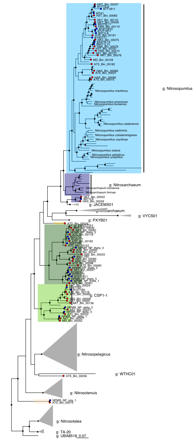
Figure 1: Phylogenomic tree
tree_nitro <- treeio::read.tree(here("NON_REDUNDANT_BINS/GTDB_tree/4_trimal_iqtree/tree_nitro_with_ref_gtdb.treefile"))

### GTDB metadata was downloaded from their release website to decorate the tree
# add taxonomy of GTDB ref sequences
taxo_gtdb <- read.table(here::here("Ref_GTDB/ar122_taxonomy_r202.tsv"), sep = "\t")
colnames(taxo_gtdb) <- c("label", "Taxonomy")
taxo_gtdb[, c(2:8)] <- colsplit(taxo_gtdb$Taxonomy, pattern = ";",
                                names = c("Domain", "Phylum", "Class", "Order", "Family", "Genus", "Species"))
taxo_gtdb <- as_tibble(taxo_gtdb)

# From the tree and summary results, I made a MAG metadata table (supplementary table S4)
amoA_presence <- read.table(here::here("NON_REDUNDANT_BINS/Trouche_et_al_Table_S4.csv"), sep = ";", header = TRUE)
amoA_presence <- as_tibble(amoA_presence)
amoA_presence <- amoA_presence[, c(1,9,11)]

# prepare table for decorating the tree
tb_nitro <- as_tibble(tree_nitro)
# adding gtdb taxonomy
tb_nitro <- dplyr::left_join(tb_nitro, taxo_gtdb)
# adding information about the presence of the Amo
tb_nitro <- dplyr::left_join(tb_nitro, amoA_presence,  by = c("label" = "MAG.name"))

# define type: external genome with publication, MAG Abyss, GTDB
tb_nitro[grep("-contigs-prefix-formatted-only", tb_nitro$label), "Type"] <- "Zhou et al (Challenger's Deep benthic)"
tb_nitro[grep("NPMR", tb_nitro$label), "Type"] <- "Kerou et al (abyssal benthic)"
tb_nitro[grep("MTA*", tb_nitro$label), "Type"] <- "Hadopelagic"
tb_nitro[grep("Bin", tb_nitro$label), "Type"] <- "MAG"
tb_nitro[is.na(tb_nitro$Type), "Type"] <- "GTDB_seq"

# make taxonomy prettier for reference strains:
tb_nitro$label_short <- tb_nitro$label
tb_nitro[tb_nitro$Type == "GTDB_seq", "label_short"] <- NA
tb_nitro[tb_nitro$Species %in% "s__Nitrosopumilus maritimus", "label_short"] <- "Nitrosopumilus maritimus"
tb_nitro[tb_nitro$Species %in% "s__Cenarchaeum symbiosum", "label_short"] <- "Cenarchaeum symbiosum"
tb_nitro[tb_nitro$Species %in% "s__Nitrosarchaeum limnae", "label_short"] <- "Nitrosarchaeum limnae"
tb_nitro[tb_nitro$Species %in% "s__Nitrosarchaeum koreense", "label_short"] <- "Nitrosarchaeum koreense"
tb_nitro[tb_nitro$Species %in% "s__Nitrosopumilus koreensis", "label_short"] <- "Nitrosopumilus koreensis"
tb_nitro[tb_nitro$Species %in% "s__Nitrosopumilus piranensis", "label_short"] <- "Nitrosopumilus piranensis"
tb_nitro[tb_nitro$Species %in% "s__Nitrosopumilus catalinensis", "label_short"] <- "Nitrosopumilus catalinensis"
tb_nitro[tb_nitro$Species %in% "s__Nitrosopumilus sediminis", "label_short"] <- "Nitrosopumilus sediminis"
tb_nitro[tb_nitro$Species %in% "s__Nitrosopumilus salaria", "label_short"] <- "Nitrosopumilus salaria"
tb_nitro[tb_nitro$Species %in% "s__Nitrosopumilus adriaticus", "label_short"] <- "Nitrosopumilus adriaticus"
tb_nitro[tb_nitro$Species %in% "s__Nitrosopumilus cobalaminigenes", "label_short"] <- "Nitrosopumilus cobalaminigenes"
tb_nitro[tb_nitro$Species %in% "s__Nitrosopumilus oxyclinae", "label_short"] <- "Nitrosopumilus oxyclinae"
tb_nitro[tb_nitro$Species %in% "s__Nitrosopumilus ureiphilus", "label_short"] <- "Nitrosopumilus ureiphilus"
tb_nitro$label_short <- gsub("-contigs-prefix-formatted-only", "", tb_nitro$label_short)
tb_nitro$label_short <- gsub("'", "", tb_nitro$label_short)

# add this table of info to the tree for plotting
tree_nitro <- full_join(tree_nitro, tb_nitro)
# I already have only o__Nitrososphaerales. Subset to AOA = family Nitrosopumilaceae
tree_NP <- tree_subset(tree_nitro, node=321, levels_back=0)

tb_NP <- as_tibble(tree_NP)

# This is how to find parent nodes
MRCA(tb_NP, 12, 14)
## # A tibble: 1 × 16
##   parent  node branch.length label group Taxonomy Phylum Class Order Family
##    <int> <int>         <dbl> <chr> <fct> <chr>    <chr>  <chr> <chr> <chr>
## 1    199   210        0.0490 100   1     <NA>     <NA>   <NA>  <NA>  <NA>
## # ℹ 6 more variables: Genus <chr>, Species <chr>, amoA.clade <chr>,
## #   Presence.of.amoA.gene <chr>, Type <chr>, label_short <chr>
MAG_nodes <- which(tb_NP$Type == "MAG")
# more precisely:
amoA_yes_nodes <- which(tb_NP$Presence.of.amoA.gene == "yes")
MAG_no_amoA <- MAG_nodes[! MAG_nodes %in% amoA_yes_nodes]

ref_nodes <- grep("prefix-formatted", tb_NP$label)

# annotate the full tree with the clades
# branch.length = "none", layout='circular': if I want it circular and no branch length
x <- ggtree(tree_NP)

p <- x +
  geom_hilight(node=250, fill="chartreuse3", alpha=0.4) + # NP-delta
  geom_hilight(node=267, fill="darkgreen", alpha=0.4) + # NP-theta
  geom_hilight(node=297, fill="deepskyblue", alpha=0.4) + # gamma 2.1, Nitrosopumilus
  geom_hilight(node=373, fill="darkblue", alpha=0.4) + # gamma 2.2, Nitrosarchaeum
  geom_hilight(node=383, fill="darkblue", alpha=0.4) + # gamma 2.2, MAGs
  geom_hilight(node=97, fill="gold", alpha=0.4) + # alpha
  geom_hilight(node=213, fill="bisque", alpha=0.4) + # iota
  geom_point2(aes(subset=(node %in% amoA_yes_nodes)), shape=23, size=2, fill='red') +
  geom_point2(aes(subset=(node %in% MAG_no_amoA)), shape=21, size=2, fill='red') +
  geom_point2(aes(subset=(node %in% ref_nodes)), shape=21, size=2, fill='blue') +
  geom_cladelabel(227, "g: Nitrosopelagicus", barsize=1, fontsize=4, offset.text = 0.2) +
  geom_cladelabel(257, "g: CSP1-1", barsize=1, fontsize=4, offset.text = 0.1) +
  geom_cladelabel(86, "g: DRGT01", barsize=1, fontsize=4) +
  geom_cladelabel(388, "g: Cenarchaeum", barsize=1, fontsize=4, offset.text = 0.1) +
  geom_cladelabel(373, "g: Nitrosarchaeum", barsize=1, fontsize=4, offset.text = 0.1) +
  geom_cladelabel(297, "g: Nitrosopumilus", barsize=1, fontsize=4, offset.text = 0.1) +
  geom_cladelabel(215, "g: Nitrosotenuis", barsize=1, fontsize=4, offset.text = 0.15) +
  geom_cladelabel(200, "g: Nitrosotalea", barsize=1, fontsize=4, offset.text = 0.1) +
  geom_cladelabel(210, "g: TA-20", barsize=1, fontsize=4, offset.text = 0.1) +
  geom_cladelabel(15, "g: UBA8516", barsize=1, fontsize=4, offset.text = 0.1) +
  geom_cladelabel(29, "g: WTHC01", barsize=1, fontsize=4, offset.text = 0.1) +
  geom_cladelabel(385, "g: JACEMX01", barsize=1, fontsize=4, offset.text = 0.1) +
  geom_cladelabel(390, "g: VYCS01", barsize=1, fontsize=4, offset.text = 0.1) +
  geom_cladelabel(391, "g: PXYB01", barsize=1, fontsize=4, offset.text = 0.1) +
  geom_tiplab(aes(label = label_short), size=3, color="black", offset = 0.01) +
  xlim(0, 1) + geom_treescale() +
  geom_nodepoint(aes(subset = !is.na(as.numeric(label)) & as.numeric(label) > 95),
                 size=1.5, color = "black", alpha = 0.9)

# plot and collapse part of the tree with no interesting MAGs
#svg(here::here("Export_figures/Nitrosopumilaceae_tree.svg"), width=10, height=20)
p  %>% collapse(node = 200, 'min', fill="grey") %>% # Nitrosotalea
  collapse(node = 227, 'min', fill="grey") %>% # Nitrosopelagicus
  collapse(node = 215, 'min', fill="grey") %>% #Nitrosotenuis
  collapse(node = 385, 'min', fill="grey") %>% # JACEMX01
  collapse(node = 390, 'min', fill="grey") %>% # VYCS01
  collapse(node = 391, 'min', fill="grey") %>% # PXYB01
  collapse(node = 388, 'min', fill="grey") %>% # Cenarchaeum
  collapse(node = 210, 'min', fill="grey") #TA-20
#dev.off()
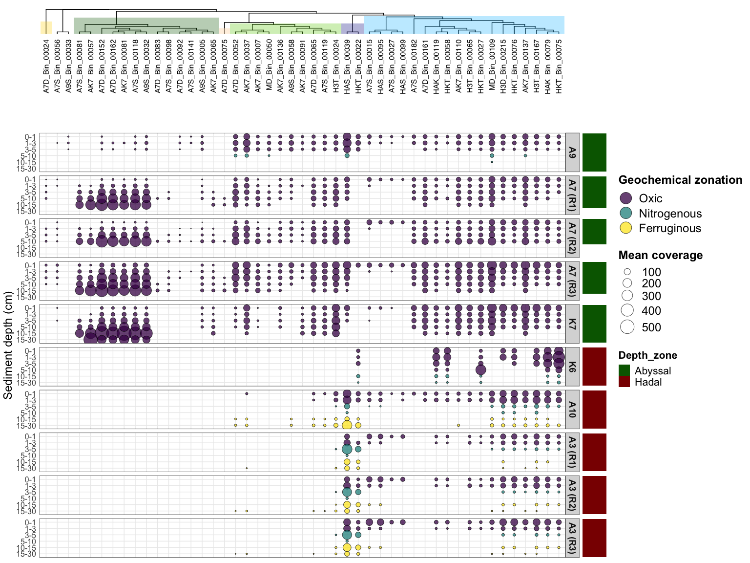
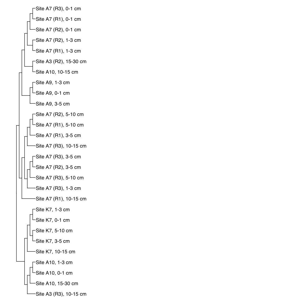
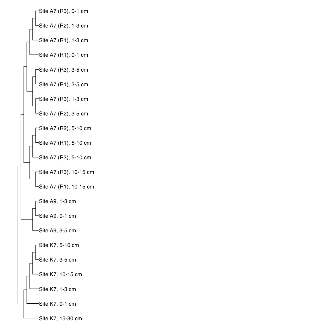
Figure 2: Mean coverage in samples, with detection threshold
# Read the mean coverage table generated by the last summary
mean_cov <- read.table(here::here("NON_REDUNDANT_BINS/07_NR-MAGs-SUMMARY/bins_across_samples/mean_coverage.txt"),
                       row.names = 1, header = TRUE)

# Read the taxonomy table derived from CheckM, GTDB, and the phylogenomic tree
taxo <- read.table(here::here("NON_REDUNDANT_BINS/Trouche_et_al_Table_S4.csv"),
                   row.names = 1, sep = ";", header = TRUE)
taxo$label <- rownames(taxo)
colnames(taxo) <- c("total_length", "num_contigs", "Longest.contig", "N50",
                    "GC_content", "percent_completion", "percent_redundancy",
                    "amoA.clade", "Presence.of.16S.gene", "Presence.of.amoA.gene",
                    "Study.accession", "Biosample", "label")

taxo_test <- read.table(here::here("03_Non_redundant_bins/03_Taxonomy/Taxo_clade_nitroso.csv"),
                   row.names = 1, sep = ";", header = TRUE)

# Read the metagenome metadata (Table S1)
meta <- read.table(here::here("Trouche_et_al_Table_S1.csv"), sep=";",
                   row.names = 1, header = TRUE)
meta$Sample_ID <- rownames(meta)

# read the "small" tree of only MAGs
tree <- treeio::read.tree(here("NON_REDUNDANT_BINS/GTDB_tree/4_trimal_iqtree_short/NR_MAGs_only_clean.fasta.treefile"))

taxo$amoA.clade != "non AOA"
##  [1] TRUE TRUE TRUE TRUE TRUE TRUE TRUE TRUE TRUE TRUE TRUE TRUE TRUE TRUE TRUE
## [16] TRUE TRUE TRUE TRUE TRUE TRUE TRUE TRUE TRUE TRUE TRUE TRUE TRUE TRUE TRUE
## [31] TRUE TRUE TRUE TRUE TRUE TRUE TRUE TRUE TRUE TRUE TRUE TRUE TRUE TRUE TRUE
## [46] TRUE TRUE
cov_nitro <- mean_cov[rownames(mean_cov) %in% rownames(taxo[taxo$amoA.clade != "non AOA",]), ]

# coverage bubble plot
cov_nitro$MAG <- rownames(cov_nitro)
cov_nitro_long <- pivot_longer(cov_nitro, c(1:56))
colnames(cov_nitro_long) <- c("MAG_name", "sample_id", "mean_coverage")
cov_nitro_long <- left_join(cov_nitro_long, meta, by = c("sample_id" = "Sample_ID"))

cov_nitro_long$Horizon <- factor(cov_nitro_long$Horizon, levels = horizon_order)
cov_nitro_long$Unique_site <- factor(cov_nitro_long$Unique_site, levels = site_order)

# Load coverage by sample for all MAGs
MAG_by_sample_cov <- read.table(here("NON_REDUNDANT_BINS/07_NR-MAGs-SUMMARY/bins_across_samples/mean_coverage.txt"),
                                header = TRUE, row.names = 1)

MAG_by_sample_cov <- as.data.frame(t(MAG_by_sample_cov))
MAG_by_sample_cov$Sample_ID <- rownames(MAG_by_sample_cov)
MAG_by_sample_cov <- left_join(MAG_by_sample_cov, meta, by = c("Sample_ID"))
MAG_by_sample_cov$Horizon <- factor(MAG_by_sample_cov$Horizon, levels = horizon_order)
detection <- read.table(here::here("NON_REDUNDANT_BINS/07_NR-MAGs-SUMMARY/bins_across_samples/detection.txt"),
                        row.names = 1, sep = "\t", header = TRUE)

detection_AOA <- detection[rownames(detection) %in% rownames(taxo[taxo$amoA.clade != "non AOA",]), ]
detection_AOA$MAG_name <- rownames(detection_AOA)
detection_AOA_long <- pivot_longer(detection_AOA, c(1:56))
colnames(detection_AOA_long) <- c("MAG_name", "sample_id", "detection")

detection_AOA_long <- left_join(detection_AOA_long, meta, by = c("sample_id" = "Sample_ID"))
detection_AOA_long[detection_AOA_long$detection >= 0.7, "detection_TF"] <-  "Over 0.7"
detection_AOA_long[detection_AOA_long$detection < 0.7, "detection_TF"] <-  "Below 0.7"

AOA_long <- left_join(detection_AOA_long, cov_nitro_long,
                      c("MAG_name", "sample_id", "Trench", "Depth_zone", "Site_depth",
                        "Horizon", "Site", "Core", "Zonation", "Unique_site", "Simple_labels"))

# create column where coverage is 0 if detection below 0.7
AOA_long$cov_by_detec <- AOA_long$mean_coverage
AOA_long[AOA_long$detection_TF == "Below 0.7", "cov_by_detec"] <- NA
# A7D_Bin_00083 and A7S_Bin_00141 only NA
samples_of_interest <- AOA_long[AOA_long$detection >= 0.7 & AOA_long$mean_coverage >= 10, ]
samples_of_interest <- samples_of_interest[,c("MAG_name", "sample_id")]
table(samples_of_interest$MAG_name)
##
## A7D_Bin_00024 A7D_Bin_00052 A7D_Bin_00065 A7D_Bin_00075 A7D_Bin_00083
##             6            23            26             5             4
## A7D_Bin_00092 A7D_Bin_00152 A7D_Bin_00161 A7D_Bin_00162 A7S_Bin_00015
##             1            20            24            19            18
## A7S_Bin_00027 A7S_Bin_00056 A7S_Bin_00081 A7S_Bin_00098 A7S_Bin_00118
##             8             2            15             4            20
## A7S_Bin_00119 A7S_Bin_00182 A9S_Bin_00005 A9S_Bin_00032 A9S_Bin_00058
##            24            19            15            22            16
## AK7_Bin_00007 AK7_Bin_00037 AK7_Bin_00057 AK7_Bin_00065 AK7_Bin_00081
##            15            26            13            14            19
## AK7_Bin_00091 AK7_Bin_00110 AK7_Bin_00136 AK7_Bin_00137 H3D_Bin_00215
##            12            25            20            35            39
## H3T_Bin_00024 H3T_Bin_00065 H3T_Bin_00167 HAK_Bin_00079 HAK_Bin_00119
##            28            30            40            42            35
## HAS_Bin_00039 HAS_Bin_00095 HAS_Bin_00099 HKT_Bin_00022 HKT_Bin_00027
##            44            16             9            26            36
## HKT_Bin_00058 HKT_Bin_00075 HKT_Bin_00076  MD_Bin_00050  MD_Bin_00109
##            29            39            39            13            35
# unique(samples_of_interest$MAG_name)

# This was done once
# i <- 1
# for (i in 1:length(unique(samples_of_interest$MAG_name))) {
#   MAG <- unique(samples_of_interest$MAG_name)[i]
#   write.table(x = samples_of_interest[samples_of_interest$MAG_name == MAG, "sample_id"],
#               file = here(paste0("NON_REDUNDANT_BINS/10_VAR_PROFILES/1_sample_files/", MAG,
#                                  "_samples_over10_over0.7.txt", sep = "")),
#               quote = FALSE, row.names = FALSE, col.names = FALSE) }
tree_nitro <- treeio::read.tree(here("NON_REDUNDANT_BINS/GTDB_tree/4_trimal_iqtree_short/NR_MAGs_only_clean.fasta.treefile"))
tb_short <- as_tibble(tree)
tb_short <- dplyr::left_join(tb_short, taxo)
tree_md <- treeio::full_join(tree, tb_short)
AOA_long$Horizon <- factor(AOA_long$Horizon, levels = flipped_horizon_order)
AOA_long$Zonation <- factor(AOA_long$Zonation, levels = c("Oxic", "Nitrogenous", "Ferruginous"))
AOA_long$Unique_site <- factor(AOA_long$Unique_site, levels = c("A9_CT1", "A7_CT1", "A7_CT2", "A7_CT3", "K7_CT5",
                                                              "K6_CT7", "A10_CT1", "A3_CT1", "A3_CT2", "A3_CT3"))

x <- ggtree(tree_md, branch.length="none", layout = "rectangular") + layout_dendrogram() +
  geom_hilight(node=62, fill="deepskyblue", alpha = 0.3) +
  geom_hilight(node=79, fill="darkblue", alpha = 0.3) +
  geom_hilight(node=52, fill="chartreuse3", alpha = 0.3) +
  geom_hilight(node=80, fill="darkgreen", alpha = 0.3) +
  geom_hilight(node=1, fill="gold", alpha = 0.3) +
  geom_hilight(node=12, fill="bisque", alpha = 0.5) +
  geom_tiplab(aes(label=label), size=4, offset=0.1, angle = 90, hjust = 1.1) +
  ggexpand(0.01, direction = 1, side = "h")

p10 <- ggplot(AOA_long, aes(x = MAG_name, y = Horizon)) +
  geom_point(aes(size = cov_by_detec, fill = Zonation), alpha = 0.75, shape = 21) +
  scale_size(range = c(.1, 10), name="Mean coverage") +
  facet_grid(Unique_site~., labeller = labeller(Unique_site = unique_site_labs)) +
  labs(fill = "Geochemical zonation") + ylab("Sediment depth (cm)") +
  scale_y_discrete(breaks = c("0_1", "1_3", "3_5", "5_10", "10_15", "15_30"),
                   labels = c("0-1", "1-3", "3-5", "5-10", "10-15", "15-30")) +
  theme_bw() +
  theme(axis.text.y = element_text(size = 12),
        axis.title.y = element_text(size = 18), axis.ticks = element_blank(),
        axis.text.x = element_blank(),
        axis.title.x = element_blank(),
        legend.title = element_text(size = 18, face = "bold"), legend.text = element_text(size = 18),
        strip.text = element_text(size = 14, face = "bold")) +
  scale_fill_viridis_d(guide = guide_legend(override.aes = list(size = 8)))


e <- ggplot(AOA_long, aes(x = 1, y = Horizon)) + geom_tile(aes(fill=Depth_zone)) +
  facet_grid(Unique_site~.) + theme_bw() +
  theme(axis.text.y = element_blank(), axis.title.y = element_blank(),
        axis.text.x = element_blank(), axis.title.x = element_blank(),
        axis.ticks = element_blank(), strip.background = element_blank(), strip.text = element_blank(),
        legend.title = element_text(size = 16, face = "bold"), legend.text = element_text(size = 16),
        panel.grid.major = element_blank(), panel.grid.minor = element_blank(),
        panel.border = element_blank()) +
  scale_fill_manual(values = scale_habitat)

q <- p10 %>% insert_top(x, height=0.3) %>%
  insert_right(e, width = 0.05)

#svg(here::here("Export_figures/Figure2.svg"), width=15, height=15)
q
#dev.off()
Figure 3: Representative FST-based trees
# HAK_Bin_00079: gamma-2.1, SNV
HAK_Bin_00079_FST <- treeio::read.tree(here("NON_REDUNDANT_BINS/10_VAR_PROFILES/3_FST_SNV/FST_HAK_Bin_00079.newick"))
FST_simple <- full_join(HAK_Bin_00079_FST, meta[meta$Sample_ID %in% HAK_Bin_00079_FST$tip.label,],
                        by = c("label" = "Sample_ID"))

x_simple <- ggtree(FST_simple, branch.length="none") +
  geom_tiplab(aes(label=Simple_labels), size=5, offset=0.1)

#svg(here::here("Export_figures/Figure3_HAK79_SNV_FST.svg"), width=10, height=12)
x_simple + xlim(0,100)
#dev.off()
HAK79_FST_txt <- read.table(here("NON_REDUNDANT_BINS/10_VAR_PROFILES/3_FST_SNV/FST_HAK_Bin_00079.txt"))
HAK79_FST_dist <- as.dist(HAK79_FST_txt)
meta_dist <- meta[meta$Sample_ID %in% colnames(HAK79_FST_txt), ]

depth.bd <- betadisper(HAK79_FST_dist, meta_dist$Depth_zone)
anova(depth.bd) # not significant: ok
## Analysis of Variance Table
##
## Response: Distances
##           Df   Sum Sq   Mean Sq F value Pr(>F)
## Groups     1 0.007038 0.0070375  1.3399 0.2539
## Residuals 40 0.210090 0.0052523
adonis2(HAK79_FST_dist~Depth_zone, data = meta_dist, permutations = 999, by = "terms")
## Permutation test for adonis under reduced model
## Terms added sequentially (first to last)
## Permutation: free
## Number of permutations: 999
##
## adonis2(formula = HAK79_FST_dist ~ Depth_zone, data = meta_dist, permutations = 999, by = "terms")
##            Df SumOfSqs      R2      F Pr(>F)
## Depth_zone  1  0.13058 0.06853 2.9431   0.02 *
## Residual   40  1.77478 0.93147
## Total      41  1.90536 1.00000
## ---
## Signif. codes:  0 '***' 0.001 '**' 0.01 '*' 0.05 '.' 0.1 ' ' 1
trench.bd <- betadisper(HAK79_FST_dist, meta_dist$Trench)
anova(trench.bd) # significant: ok
## Analysis of Variance Table
##
## Response: Distances
##           Df   Sum Sq  Mean Sq F value    Pr(>F)
## Groups     1 0.064762 0.064762  13.196 0.0007895 ***
## Residuals 40 0.196311 0.004908
## ---
## Signif. codes:  0 '***' 0.001 '**' 0.01 '*' 0.05 '.' 0.1 ' ' 1
TukeyHSD(trench.bd)
##   Tukey multiple comparisons of means
##     95% family-wise confidence level
##
## Fit: aov(formula = distances ~ group, data = df)
##
## $group
##                         diff        lwr         upr     p adj
## Kermadec-Atacama -0.09219536 -0.1434902 -0.04090047 0.0007895
adonis2(HAK79_FST_dist~Depth_zone*Trench, data = meta_dist, permutations = 999, by = "terms")
## Permutation test for adonis under reduced model
## Terms added sequentially (first to last)
## Permutation: free
## Number of permutations: 999
##
## adonis2(formula = HAK79_FST_dist ~ Depth_zone * Trench, data = meta_dist, permutations = 999, by = "terms")
##                   Df SumOfSqs      R2      F Pr(>F)
## Depth_zone         1  0.13058 0.06853 3.3839  0.008 **
## Trench             1  0.25679 0.13477 6.6545  0.001 ***
## Depth_zone:Trench  1  0.05157 0.02707 1.3365  0.188
## Residual          38  1.46641 0.76962
## Total             41  1.90536 1.00000
## ---
## Signif. codes:  0 '***' 0.001 '**' 0.01 '*' 0.05 '.' 0.1 ' ' 1
### HADAL SUBSET
# it is difficult to properly nest the permanova so I will subsample
meta_dist_hadal <- meta_dist[meta_dist$Depth_zone == "Hadal",]
HAK79_FST_dist_hadal <- as.dist(HAK79_FST_txt[colnames(HAK79_FST_txt) %in% meta_dist_hadal$Sample_ID,
                                       rownames(HAK79_FST_txt) %in% meta_dist_hadal$Sample_ID])

trench.bd <- betadisper(HAK79_FST_dist_hadal, meta_dist_hadal$Trench)
anova(trench.bd) # significant
## Analysis of Variance Table
##
## Response: Distances
##           Df   Sum Sq  Mean Sq F value  Pr(>F)
## Groups     1 0.033193 0.033193  5.6892 0.02657 *
## Residuals 21 0.122520 0.005834
## ---
## Signif. codes:  0 '***' 0.001 '**' 0.01 '*' 0.05 '.' 0.1 ' ' 1
TukeyHSD(trench.bd)
##   Tukey multiple comparisons of means
##     95% family-wise confidence level
##
## Fit: aov(formula = distances ~ group, data = df)
##
## $group
##                         diff        lwr         upr     p adj
## Kermadec-Atacama -0.08651377 -0.1619432 -0.01108435 0.0265709
# group A3 + A10
meta_dist_hadalA <- meta_dist[meta_dist$Depth_zone == "Hadal" & meta_dist$Trench == "Atacama" ,]
HAK79_FST_dist_hadalA <- as.dist(HAK79_FST_txt[colnames(HAK79_FST_txt) %in% meta_dist_hadalA$Sample_ID,
                                       rownames(HAK79_FST_txt) %in% meta_dist_hadalA$Sample_ID])

horizon.bd <- betadisper(HAK79_FST_dist_hadalA, meta_dist_hadalA$Horizon)
anova(horizon.bd) # significant
## Analysis of Variance Table
##
## Response: Distances
##           Df   Sum Sq  Mean Sq F value  Pr(>F)
## Groups     4 0.023556 0.005889  3.7343 0.03382 *
## Residuals 12 0.018924 0.001577
## ---
## Signif. codes:  0 '***' 0.001 '**' 0.01 '*' 0.05 '.' 0.1 ' ' 1
TukeyHSD(horizon.bd) # but no comparison here is significant
##   Tukey multiple comparisons of means
##     95% family-wise confidence level
##
## Fit: aov(formula = distances ~ group, data = df)
##
## $group
##                    diff         lwr          upr     p adj
## 1_3-0_1      0.07682623 -0.01267860  0.166331060 0.1062075
## 10_15-0_1    0.02966347 -0.05984136  0.119168294 0.8246083
## 15_30-0_1   -0.07197520 -0.21349476  0.069544360 0.5123860
## 3_5-0_1      0.04424644 -0.04525839  0.133751266 0.5379366
## 10_15-1_3   -0.04716277 -0.13666759  0.042342063 0.4801194
## 15_30-1_3   -0.14880143 -0.29032099 -0.007281872 0.0378013
## 3_5-1_3     -0.03257979 -0.12208462  0.056925034 0.7726743
## 15_30-10_15 -0.10163867 -0.24315823  0.039880894 0.2136579
## 3_5-10_15    0.01458297 -0.07492186  0.104087800 0.9836768
## 3_5-15_30    0.11622164 -0.02529792  0.257741197 0.1285472
site.bd <- betadisper(HAK79_FST_dist_hadalA, meta_dist_hadalA$Site)
anova(site.bd) # not significant
## Analysis of Variance Table
##
## Response: Distances
##           Df    Sum Sq   Mean Sq F value Pr(>F)
## Groups     1 0.0017873 0.0017873  1.4959 0.2402
## Residuals 15 0.0179217 0.0011948
adonis2(HAK79_FST_dist_hadalA~Horizon*Site, data = meta_dist_hadalA, permutations = 999, by = "terms")
## Permutation test for adonis under reduced model
## Terms added sequentially (first to last)
## Permutation: free
## Number of permutations: 999
##
## adonis2(formula = HAK79_FST_dist_hadalA ~ Horizon * Site, data = meta_dist_hadalA, permutations = 999, by = "terms")
##              Df SumOfSqs      R2      F Pr(>F)
## Horizon       4  0.14188 0.39547 2.7334  0.001 ***
## Site          1  0.04673 0.13024 3.6007  0.001 ***
## Horizon:Site  3  0.06635 0.18493 1.7043  0.023 *
## Residual      8  0.10381 0.28936
## Total        16  0.35877 1.00000
## ---
## Signif. codes:  0 '***' 0.001 '**' 0.01 '*' 0.05 '.' 0.1 ' ' 1
### ABYSSAL SUBSET
meta_dist_abyssal <- meta_dist[meta_dist$Depth_zone == "Abyssal",]
HAK79_FST_dist_abyssal <- as.dist(HAK79_FST_txt[colnames(HAK79_FST_txt) %in% meta_dist_abyssal$Sample_ID,
                                       rownames(HAK79_FST_txt) %in% meta_dist_abyssal$Sample_ID])

horizon.bd <- betadisper(HAK79_FST_dist_abyssal, meta_dist_abyssal$Horizon)
anova(horizon.bd) # significant
## Analysis of Variance Table
##
## Response: Distances
##           Df    Sum Sq   Mean Sq F value Pr(>F)
## Groups     3 0.0053603 0.0017868   0.919 0.4554
## Residuals 15 0.0291625 0.0019442
TukeyHSD(horizon.bd) # but no comparison here is significant (except 3-5, 1-3)
##   Tukey multiple comparisons of means
##     95% family-wise confidence level
##
## Fit: aov(formula = distances ~ group, data = df)
##
## $group
##                 diff         lwr        upr     p adj
## 1_3-0_1  -0.01448328 -0.09485677 0.06589020 0.9531302
## 3_5-0_1   0.01749317 -0.06288032 0.09786665 0.9216704
## 5_10-0_1  0.03076188 -0.05448708 0.11601083 0.7293276
## 3_5-1_3   0.03197645 -0.04839704 0.11234994 0.6676566
## 5_10-1_3  0.04524516 -0.04000380 0.13049411 0.4453934
## 5_10-3_5  0.01326871 -0.07198025 0.09851766 0.9688862
trench.bd <- betadisper(HAK79_FST_dist_abyssal, meta_dist_abyssal$Trench)
anova(trench.bd) # not significant
## Analysis of Variance Table
##
## Response: Distances
##           Df   Sum Sq    Mean Sq F value Pr(>F)
## Groups     1 0.000032 0.00003214  0.0172 0.8971
## Residuals 17 0.031691 0.00186418
site.bd <- betadisper(HAK79_FST_dist_abyssal, meta_dist_abyssal$Site)
anova(site.bd) # not significant
## Analysis of Variance Table
##
## Response: Distances
##           Df   Sum Sq   Mean Sq F value Pr(>F)
## Groups     2 0.002041 0.0010203  0.4269 0.6597
## Residuals 16 0.038239 0.0023899
adonis2(HAK79_FST_dist_abyssal~Horizon, data = meta_dist_abyssal, permutations = 999, by = "terms")
## Permutation test for adonis under reduced model
## Terms added sequentially (first to last)
## Permutation: free
## Number of permutations: 999
##
## adonis2(formula = HAK79_FST_dist_abyssal ~ Horizon, data = meta_dist_abyssal, permutations = 999, by = "terms")
##          Df SumOfSqs      R2      F Pr(>F)
## Horizon   3 0.082137 0.29215 2.0637  0.024 *
## Residual 15 0.199007 0.70785
## Total    18 0.281144 1.00000
## ---
## Signif. codes:  0 '***' 0.001 '**' 0.01 '*' 0.05 '.' 0.1 ' ' 1
adonis2(HAK79_FST_dist_abyssal~Trench, data = meta_dist_abyssal, permutations = 999, by = "terms")
## Permutation test for adonis under reduced model
## Terms added sequentially (first to last)
## Permutation: free
## Number of permutations: 999
##
## adonis2(formula = HAK79_FST_dist_abyssal ~ Trench, data = meta_dist_abyssal, permutations = 999, by = "terms")
##          Df SumOfSqs      R2      F Pr(>F)
## Trench    1 0.027426 0.09755 1.8376  0.106
## Residual 17 0.253718 0.90245
## Total    18 0.281144 1.00000
adonis2(HAK79_FST_dist_abyssal~Site, data = meta_dist_abyssal, permutations = 999, by = "terms")
## Permutation test for adonis under reduced model
## Terms added sequentially (first to last)
## Permutation: free
## Number of permutations: 999
##
## adonis2(formula = HAK79_FST_dist_abyssal ~ Site, data = meta_dist_abyssal, permutations = 999, by = "terms")
##          Df SumOfSqs      R2     F Pr(>F)
## Site      2 0.034282 0.12194 1.111  0.335
## Residual 16 0.246862 0.87806
## Total    18 0.281144 1.00000
# HAS_Bin_00039: gamma-2.1, SNV
HAS_Bin_00039_FST <- treeio::read.tree(here("NON_REDUNDANT_BINS/10_VAR_PROFILES/3_FST_SNV/FST_HAS_Bin_00039.newick"))
FST_simple <- full_join(HAS_Bin_00039_FST, meta[meta$Sample_ID %in% HAS_Bin_00039_FST$tip.label,],
                        by = c("label" = "Sample_ID"))

x_simple <- ggtree(FST_simple, branch.length="none") +
  geom_tiplab(aes(label=Simple_labels), size=5, offset=0.1)

#svg(here::here("Export_figures/Figure3_HAS39_SNV_FST.svg"), width=10, height=12)
x_simple + xlim(0,100)
#dev.off()
HAS39_FST_txt <- read.table(here("NON_REDUNDANT_BINS/10_VAR_PROFILES/3_FST_SNV/FST_HAS_Bin_00039.txt"))
HAS39_FST_dist <- as.dist(HAS39_FST_txt)
meta_dist <- meta[meta$Sample_ID %in% colnames(HAS39_FST_txt), ]

depth.bd <- betadisper(HAS39_FST_dist, meta_dist$Depth_zone)
anova(depth.bd) # significant, this might influence the result
## Analysis of Variance Table
##
## Response: Distances
##           Df   Sum Sq  Mean Sq F value   Pr(>F)
## Groups     1 0.043298 0.043298  7.6912 0.008242 **
## Residuals 42 0.236440 0.005630
## ---
## Signif. codes:  0 '***' 0.001 '**' 0.01 '*' 0.05 '.' 0.1 ' ' 1
TukeyHSD(depth.bd)
##   Tukey multiple comparisons of means
##     95% family-wise confidence level
##
## Fit: aov(formula = distances ~ group, data = df)
##
## $group
##                      diff        lwr         upr     p adj
## Hadal-Abyssal -0.06299953 -0.1088433 -0.01715577 0.0082416
adonis2(HAS39_FST_dist~Depth_zone, data = meta_dist, permutations = 999, by = "terms")
## Permutation test for adonis under reduced model
## Terms added sequentially (first to last)
## Permutation: free
## Number of permutations: 999
##
## adonis2(formula = HAS39_FST_dist ~ Depth_zone, data = meta_dist, permutations = 999, by = "terms")
##            Df SumOfSqs      R2      F Pr(>F)
## Depth_zone  1  0.62111 0.27531 15.956  0.001 ***
## Residual   42  1.63491 0.72469
## Total      43  2.25602 1.00000
## ---
## Signif. codes:  0 '***' 0.001 '**' 0.01 '*' 0.05 '.' 0.1 ' ' 1
# The adonis result reflects the heterogeneity of the samples.
# However here we have compositional data based on variants, which means that if we are heterogeneous, we are proving that we have differing populations as well.

### HADAL CLUSTER
meta_dist_hadal <- meta_dist[meta_dist$Depth_zone == "Hadal",]
HAS39_FST_dist_hadal <- as.dist(HAS39_FST_txt[colnames(HAS39_FST_txt) %in% meta_dist_hadal$Sample_ID,
                                       rownames(HAS39_FST_txt) %in% meta_dist_hadal$Sample_ID])

horizon.bd <- betadisper(HAS39_FST_dist_hadal, meta_dist_hadal$Horizon)
anova(horizon.bd) # not significant
## Analysis of Variance Table
##
## Response: Distances
##           Df   Sum Sq   Mean Sq F value  Pr(>F)
## Groups     5 0.051955 0.0103910  2.5509 0.06501 .
## Residuals 18 0.073321 0.0040734
## ---
## Signif. codes:  0 '***' 0.001 '**' 0.01 '*' 0.05 '.' 0.1 ' ' 1
site.bd <- betadisper(HAS39_FST_dist_hadal, meta_dist_hadal$Site)
anova(site.bd) # not significant
## Analysis of Variance Table
##
## Response: Distances
##           Df   Sum Sq   Mean Sq F value Pr(>F)
## Groups     1 0.002993 0.0029930  0.6444 0.4307
## Residuals 22 0.102188 0.0046449
adonis2(HAS39_FST_dist_hadal~Horizon*Site, data = meta_dist_hadal, permutations = 999, by = "terms")
## Permutation test for adonis under reduced model
## Terms added sequentially (first to last)
## Permutation: free
## Number of permutations: 999
##
## adonis2(formula = HAS39_FST_dist_hadal ~ Horizon * Site, data = meta_dist_hadal, permutations = 999, by = "terms")
##              Df SumOfSqs      R2      F Pr(>F)
## Horizon       5  0.12326 0.25407 2.1669  0.001 ***
## Site          1  0.11140 0.22961 9.7915  0.001 ***
## Horizon:Site  5  0.11397 0.23492 2.0035  0.028 *
## Residual     12  0.13652 0.28140
## Total        23  0.48516 1.00000
## ---
## Signif. codes:  0 '***' 0.001 '**' 0.01 '*' 0.05 '.' 0.1 ' ' 1
### ABYSSAL CLUSTER
meta_dist_abyssal <- meta_dist[meta_dist$Depth_zone == "Abyssal",]
HAS39_FST_dist_abyssal <- as.dist(HAS39_FST_txt[colnames(HAS39_FST_txt) %in% meta_dist_abyssal$Sample_ID,
                                       rownames(HAS39_FST_txt) %in% meta_dist_abyssal$Sample_ID])

site.bd <- betadisper(HAS39_FST_dist_abyssal, meta_dist_abyssal$Site)
anova(site.bd) # not significant
## Analysis of Variance Table
##
## Response: Distances
##           Df   Sum Sq   Mean Sq F value Pr(>F)
## Groups     2 0.008345 0.0041723  0.9138 0.4198
## Residuals 17 0.077625 0.0045662
adonis2(HAS39_FST_dist_abyssal~Trench, data = meta_dist_abyssal, permutations = 999, by = "terms")
## Permutation test for adonis under reduced model
## Terms added sequentially (first to last)
## Permutation: free
## Number of permutations: 999
##
## adonis2(formula = HAS39_FST_dist_abyssal ~ Trench, data = meta_dist_abyssal, permutations = 999, by = "terms")
##          Df SumOfSqs      R2      F Pr(>F)
## Trench    1  0.12849 0.15685 3.3485  0.002 **
## Residual 18  0.69072 0.84315
## Total    19  0.81921 1.00000
## ---
## Signif. codes:  0 '***' 0.001 '**' 0.01 '*' 0.05 '.' 0.1 ' ' 1
adonis2(HAS39_FST_dist_abyssal~Site, data = meta_dist_abyssal, permutations = 9999, by = "terms")
## Permutation test for adonis under reduced model
## Terms added sequentially (first to last)
## Permutation: free
## Number of permutations: 9999
##
## adonis2(formula = HAS39_FST_dist_abyssal ~ Site, data = meta_dist_abyssal, permutations = 9999, by = "terms")
##          Df SumOfSqs      R2      F Pr(>F)
## Site      2  0.17273 0.21085 2.2711  0.002 **
## Residual 17  0.64648 0.78915
## Total    19  0.81921 1.00000
## ---
## Signif. codes:  0 '***' 0.001 '**' 0.01 '*' 0.05 '.' 0.1 ' ' 1
## Abyssal atacama
meta_dist_abyssalA <- meta_dist[meta_dist$Site == "A7",]
HAS39_FST_dist_abyssalA <- as.dist(HAS39_FST_txt[colnames(HAS39_FST_txt) %in% meta_dist_abyssalA$Sample_ID,
                                       rownames(HAS39_FST_txt) %in% meta_dist_abyssalA$Sample_ID])

horizon.bd <- betadisper(HAS39_FST_dist_abyssalA, meta_dist_abyssalA$Horizon)
anova(horizon.bd) # not significant
## Analysis of Variance Table
##
## Response: Distances
##           Df   Sum Sq   Mean Sq F value Pr(>F)
## Groups     4 0.029391 0.0073479  1.6077 0.2628
## Residuals  8 0.036563 0.0045704
adonis2(HAS39_FST_dist_abyssalA~Horizon, data = meta_dist_abyssalA, permutations = 999, by = "terms")
## Permutation test for adonis under reduced model
## Terms added sequentially (first to last)
## Permutation: free
## Number of permutations: 999
##
## adonis2(formula = HAS39_FST_dist_abyssalA ~ Horizon, data = meta_dist_abyssalA, permutations = 999, by = "terms")
##          Df SumOfSqs     R2      F Pr(>F)
## Horizon   4  0.18207 0.4416 1.5817  0.042 *
## Residual  8  0.23023 0.5584
## Total    12  0.41230 1.0000
## ---
## Signif. codes:  0 '***' 0.001 '**' 0.01 '*' 0.05 '.' 0.1 ' ' 1
# H3T_Bin_00024: gamma-2.1, SNV
H3T_Bin_00024_FST <- treeio::read.tree(here("NON_REDUNDANT_BINS/10_VAR_PROFILES/3_FST_SNV/FST_H3T_Bin_00024.newick"))
FST_simple <- full_join(H3T_Bin_00024_FST, meta[meta$Sample_ID %in% H3T_Bin_00024_FST$tip.label,],
                        by = c("label" = "Sample_ID"))

x_simple <- ggtree(FST_simple, branch.length="none") +
  geom_tiplab(aes(label=Simple_labels), size=5, offset=0.1)

#svg(here::here("Export_figures/Figure3_H3T24_SNV_FST.svg"), width=10, height=12)
x_simple + xlim(0,100)
#dev.off()
H3T24_FST_txt <- read.table(here("NON_REDUNDANT_BINS/10_VAR_PROFILES/3_FST_SNV/FST_H3T_Bin_00024.txt"))
H3T24_FST_dist <- as.dist(H3T24_FST_txt)
meta_dist <- meta[meta$Sample_ID %in% colnames(H3T24_FST_txt), ]

site.bd <- betadisper(H3T24_FST_dist, meta_dist$Site)
anova(site.bd) # not significant
## Analysis of Variance Table
##
## Response: Distances
##           Df   Sum Sq   Mean Sq F value Pr(>F)
## Groups     4 0.033009 0.0082524  1.8779 0.1486
## Residuals 23 0.101075 0.0043945
trench.bd <- betadisper(H3T24_FST_dist, meta_dist$Site)
anova(site.bd) # not significant
## Analysis of Variance Table
##
## Response: Distances
##           Df   Sum Sq   Mean Sq F value Pr(>F)
## Groups     4 0.033009 0.0082524  1.8779 0.1486
## Residuals 23 0.101075 0.0043945
adonis2(H3T24_FST_dist~Site, data = meta_dist, permutations = 999, by = "terms")
## Permutation test for adonis under reduced model
## Terms added sequentially (first to last)
## Permutation: free
## Number of permutations: 999
##
## adonis2(formula = H3T24_FST_dist ~ Site, data = meta_dist, permutations = 999, by = "terms")
##          Df SumOfSqs      R2      F Pr(>F)
## Site      4  0.36067 0.36638 3.3248  0.001 ***
## Residual 23  0.62376 0.63362
## Total    27  0.98444 1.00000
## ---
## Signif. codes:  0 '***' 0.001 '**' 0.01 '*' 0.05 '.' 0.1 ' ' 1
adonis2(H3T24_FST_dist~Trench, data = meta_dist, permutations = 999, by = "terms")
## Permutation test for adonis under reduced model
## Terms added sequentially (first to last)
## Permutation: free
## Number of permutations: 999
##
## adonis2(formula = H3T24_FST_dist ~ Trench, data = meta_dist, permutations = 999, by = "terms")
##          Df SumOfSqs      R2      F Pr(>F)
## Trench    1  0.13018 0.13224 3.9622  0.001 ***
## Residual 26  0.85425 0.86776
## Total    27  0.98444 1.00000
## ---
## Signif. codes:  0 '***' 0.001 '**' 0.01 '*' 0.05 '.' 0.1 ' ' 1
# it is difficult to properly nest the permanova so I will subsample to abyssal atacama
meta_dist_abyssalA <- meta_dist[meta_dist$Depth_zone == "Abyssal" & meta_dist$Trench == "Atacama",]
H3T24_FST_dist_abyssalA <- as.dist(H3T24_FST_txt[colnames(H3T24_FST_txt) %in% meta_dist_abyssalA$Sample_ID,
                                       rownames(H3T24_FST_txt) %in% meta_dist_abyssalA$Sample_ID])

horizon.bd <- betadisper(H3T24_FST_dist_abyssalA, meta_dist_abyssalA$Horizon)
anova(horizon.bd) # not significant
## Analysis of Variance Table
##
## Response: Distances
##           Df   Sum Sq   Mean Sq F value Pr(>F)
## Groups     4 0.019827 0.0049566  0.7461  0.579
## Residuals 12 0.079721 0.0066434
adonis2(H3T24_FST_dist_abyssalA~Horizon*Site, data = meta_dist_abyssalA, permutations = 999, by = "terms")
## Permutation test for adonis under reduced model
## Terms added sequentially (first to last)
## Permutation: free
## Number of permutations: 999
##
## adonis2(formula = H3T24_FST_dist_abyssalA ~ Horizon * Site, data = meta_dist_abyssalA, permutations = 999, by = "terms")
##              Df SumOfSqs      R2       F Pr(>F)
## Horizon       4  0.13143 0.34019  4.1918  0.002 **
## Site          1  0.15303 0.39612 19.5238  0.001 ***
## Horizon:Site  2  0.03133 0.08108  1.9982  0.128
## Residual      9  0.07054 0.18260
## Total        16  0.38633 1.00000
## ---
## Signif. codes:  0 '***' 0.001 '**' 0.01 '*' 0.05 '.' 0.1 ' ' 1
# A9S_Bin_00032: gamma-2.1, SNV
A9S_Bin_00032_FST <- treeio::read.tree(here("NON_REDUNDANT_BINS/10_VAR_PROFILES/3_FST_SNV/FST_A9S_Bin_00032.newick"))
FST_simple <- full_join(A9S_Bin_00032_FST, meta[meta$Sample_ID %in% A9S_Bin_00032_FST$tip.label,],
                        by = c("label" = "Sample_ID"))
x_simple <- ggtree(FST_simple, branch.length="none") +
  geom_tiplab(aes(label=Simple_labels), size=5, offset=0.1)

#svg(here::here("Export_figures/Figure3_AS932_SNV_FST.svg"), width=10, height=12)
x_simple + xlim(0,100)
#dev.off()
A9S32_FST_txt <- read.table(here("NON_REDUNDANT_BINS/10_VAR_PROFILES/3_FST_SNV/FST_A9S_Bin_00032.txt"))
A9S32_FST_dist <- as.dist(A9S32_FST_txt)
meta_dist <- meta[meta$Sample_ID %in% colnames(A9S32_FST_txt), ]

site.bd <- betadisper(A9S32_FST_dist, meta_dist$Site)
anova(site.bd) # not significant
## Analysis of Variance Table
##
## Response: Distances
##           Df   Sum Sq   Mean Sq F value Pr(>F)
## Groups     2 0.015509 0.0077543  2.4137 0.1164
## Residuals 19 0.061039 0.0032126
adonis2(A9S32_FST_dist~Site, data = meta_dist, permutations = 9999, by = "terms")
## Permutation test for adonis under reduced model
## Terms added sequentially (first to last)
## Permutation: free
## Number of permutations: 9999
##
## adonis2(formula = A9S32_FST_dist ~ Site, data = meta_dist, permutations = 9999, by = "terms")
##          Df SumOfSqs      R2      F Pr(>F)
## Site      2  0.13182 0.17592 2.0281 0.0349 *
## Residual 19  0.61748 0.82408
## Total    21  0.74930 1.00000
## ---
## Signif. codes:  0 '***' 0.001 '**' 0.01 '*' 0.05 '.' 0.1 ' ' 1
# it is difficult to properly nest the permanova so I will subsample to A7
meta_dist_abyssalA <- meta_dist[meta_dist$Site == "A7",]
A9S32_FST_dist_abyssalA <- as.dist(A9S32_FST_txt[colnames(A9S32_FST_txt) %in% meta_dist_abyssalA$Sample_ID,
                                       rownames(A9S32_FST_txt) %in% meta_dist_abyssalA$Sample_ID])

horizon.bd <- betadisper(A9S32_FST_dist_abyssalA, meta_dist_abyssalA$Horizon)
anova(horizon.bd) # not significant
## Analysis of Variance Table
##
## Response: Distances
##           Df    Sum Sq   Mean Sq F value Pr(>F)
## Groups     4 0.0081542 0.0020385  0.9864 0.4669
## Residuals  8 0.0165327 0.0020666
adonis2(A9S32_FST_dist_abyssalA~Horizon, data = meta_dist_abyssalA, permutations = 999, by = "terms")
## Permutation test for adonis under reduced model
## Terms added sequentially (first to last)
## Permutation: free
## Number of permutations: 999
##
## adonis2(formula = A9S32_FST_dist_abyssalA ~ Horizon, data = meta_dist_abyssalA, permutations = 999, by = "terms")
##          Df SumOfSqs      R2      F Pr(>F)
## Horizon   4 0.091152 0.47772 1.8293  0.066 .
## Residual  8 0.099655 0.52228
## Total    12 0.190807 1.00000
## ---
## Signif. codes:  0 '***' 0.001 '**' 0.01 '*' 0.05 '.' 0.1 ' ' 1
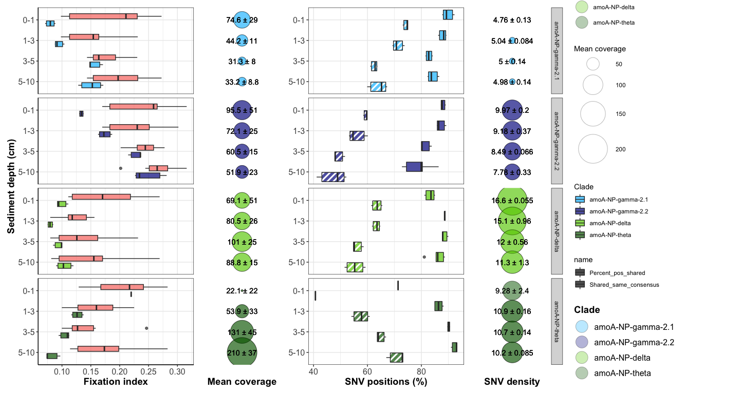
Figure 4: Downcore evolution of FST and SNV number
clade_representative_list <- c("HAK_Bin_00079", "HAS_Bin_00039", "H3T_Bin_00024", "A9S_Bin_00032")
clade_list <- c("amoA-NP-gamma-2.1", "amoA-NP-gamma-2.2", "amoA-NP-delta", "amoA-NP-theta")
scale_downcore <- c("Same core, different horizons" = "#F8766D", "Different cores, same horizon" = "#00BFC4")

downcore_plot <- function(MAG, clade){
  FST_dists <- read.table(here(paste0("NON_REDUNDANT_BINS/10_VAR_PROFILES/3_FST_SNV/FST_", MAG, ".txt")),
                          sep="\t", header=TRUE, row.names=1)

  ### triplicate vs downcore for site A7
  FST_A7 <-  FST_dists[rownames(FST_dists) %in% meta[meta$Site == "A7", "Sample_ID"],
                       colnames(FST_dists) %in% meta[meta$Site == "A7", "Sample_ID"]]
  FST_A7$Sample_ID <- rownames(FST_A7)
  FST_A7_long <- pivot_longer(FST_A7, cols = c(1:dim(FST_A7)[1]))

  # remove comparison of same sample
  FST_A7_long <- FST_A7_long[FST_A7_long$Sample_ID != FST_A7_long$name,]

  # modify colnames
  colnames(FST_A7_long) <- c("Sample_1", "Sample_2", "FST")

  FST_A7_long$Sample1_horizon = meta[match(FST_A7_long$Sample_1, rownames(meta)), "Horizon"]
  FST_A7_long$Sample2_horizon = meta[match(FST_A7_long$Sample_2, rownames(meta)), "Horizon"]
  FST_A7_long$Sample1_horizon <- factor(FST_A7_long$Sample1_horizon, levels = horizon_order)

  # add comparison type
  FST_A7_long[FST_A7_long$Sample2_horizon == FST_A7_long$Sample1_horizon, "Comparison"] <- "Different cores, same horizon"
  FST_A7_long[FST_A7_long$Sample2_horizon != FST_A7_long$Sample1_horizon, "Comparison"] <- "Same core, different horizons"

  # keep Same core, different horizons comparisons only in the same core
  FST_A7_long$Sample1_core = meta[match(FST_A7_long$Sample_1, rownames(meta)), "Core"]
  FST_A7_long$Sample2_core = meta[match(FST_A7_long$Sample_2, rownames(meta)), "Core"]
  FST_A7_long <- FST_A7_long[FST_A7_long$Comparison == "Different cores, same horizon" |
                               (FST_A7_long$Comparison == "Same core, different horizons" &
                                  FST_A7_long$Sample1_core == FST_A7_long$Sample2_core), ]

  # add MAG name and clade
  FST_A7_long$MAG_name <- MAG
  FST_A7_long$Clade <- clade
  FST_A7_long$Sample1_horizon <- factor(FST_A7_long$Sample1_horizon, levels = flipped_horizon_order)

  ## adding line of mean MAG coverage
  x <- which(colnames(MAG_by_sample_cov) == MAG)
  df_cov_by_sample <- MAG_by_sample_cov[, c(x, 91:ncol(MAG_by_sample_cov))]
  colnames(df_cov_by_sample)[1] <- "Mean_coverage"
  df_cov_by_sample_A7 <- df_cov_by_sample[df_cov_by_sample$Site == "A7", ]
  df_cov_by_sample_A7$Horizon <- factor(df_cov_by_sample_A7$Horizon, levels = flipped_horizon_order)

  ### composite plot
  df_cov_by_horizon <- df_cov_by_sample_A7 %>%
    group_by(Horizon) %>%
    dplyr::summarize(mean = signif(mean(Mean_coverage), 3), sd = signif(sd(Mean_coverage), 2)) %>%
    rename(mean_coverage = mean, coverage_sd = sd)

  df_cov_by_horizon$Horizon <- factor(df_cov_by_horizon$Horizon, levels = flipped_horizon_order)

  df_cov_by_sample_A7 <- left_join(df_cov_by_sample_A7, df_cov_by_horizon, by = c("Horizon"))
  df_cov_by_sample_A7$label <- paste0(df_cov_by_sample_A7$mean_coverage, " ± ",
                                      df_cov_by_sample_A7$coverage_sd)
  df_cov_by_sample_A7$MAG_name <- MAG
  df_cov_by_sample_A7$Clade <- clade

  return(list(FST_A7_long, df_cov_by_sample_A7))
}

FST_A7_long_full <- data.frame(matrix(ncol=0,nrow=0))
df_cov_by_sample_A7_full <- data.frame(matrix(ncol=0,nrow=0))

for(i in (1:length(clade_representative_list))){
   df_list <- downcore_plot(clade_representative_list[i], clade_list[i])
   FST_A7_long_full <- rbind(FST_A7_long_full, df_list[[1]])
   df_cov_by_sample_A7_full <- rbind(df_cov_by_sample_A7_full, df_list[[2]])
}


FST_A7_long_full$Comparison_color <- paste0(FST_A7_long_full$Comparison, " ", FST_A7_long_full$Clade)
scale_comparison <- c("Same core, different horizons amoA-NP-gamma-2.1" = "#F8766D",
                      "Same core, different horizons amoA-NP-gamma-2.2" = "#F8766D",
                      "Same core, different horizons amoA-NP-delta" = "#F8766D",
                      "Same core, different horizons amoA-NP-theta" = "#F8766D",
                      "Different cores, same horizon amoA-NP-gamma-2.1" = "deepskyblue",
                      "Different cores, same horizon amoA-NP-gamma-2.2" = "darkblue",
                      "Different cores, same horizon amoA-NP-delta" = "chartreuse3",
                      "Different cores, same horizon amoA-NP-theta" = "darkgreen")

FST_A7_long_full$Clade <- factor(FST_A7_long_full$Clade, levels = clade_list)
df_cov_by_sample_A7_full$Clade <- factor(df_cov_by_sample_A7_full$Clade, levels = clade_list)

# try withou 10-15 cm layer
FST_A7_long_full <- FST_A7_long_full[FST_A7_long_full$Sample1_horizon != "10_15" &
                                       FST_A7_long_full$Sample2_horizon != "10_15", ]
df_cov_by_sample_A7_full <- df_cov_by_sample_A7_full[df_cov_by_sample_A7_full$Horizon != "10_15",]

# by horizon type
box <- ggplot(FST_A7_long_full, aes(x = Sample1_horizon, y = FST, fill = Comparison_color)) +
  geom_boxplot(width = 0.5, linewidth = 0.5, position = position_dodge(0.7), alpha = 0.7) +
  facet_grid(Clade~.) +
  scale_x_discrete(breaks = flipped_horizon_order, labels = flipped_horizon_names) +
  xlab("Sediment depth (cm)") + ylab("Fixation index") +
  scale_fill_manual(values = scale_comparison) +
  theme_bw() +
  theme(axis.title.x = element_text(face = "bold", size = 14),
        axis.title.y = element_text(face = "bold", size = 14),
        axis.text.x = element_text(size = 12),
        axis.text.y = element_text(size = 12),
        axis.line.y = element_line(colour = "black"),
        axis.line.x = element_line(colour = "black"),
        strip.text = element_blank()) +
  coord_flip()

bubble <- ggplot(df_cov_by_sample_A7_full, aes(x = Horizon, y = factor(Site))) +
  geom_point(aes(size = mean_coverage, fill = Clade), alpha = 0.3, shape = 21) +
  facet_grid(Clade~.) +
  geom_text(aes(label = label)) +
  scale_size(range = c(1, 20), name="Mean coverage") +
  ylab("Mean coverage") + scale_fill_manual(values = scale_amoA, guide = guide_legend(override.aes = list(size = 8))) +
  theme_bw() +
  theme(axis.title.x = element_text(face = "bold", size = 14),
        axis.title.y = element_blank(),
        axis.text = element_blank(),
        panel.grid = element_blank(),
        panel.border = element_blank(),
        axis.line = element_blank(),
        axis.ticks = element_blank(),
        strip.text = element_blank()) +
  coord_flip()
## amoA-NP-gamma-2.1: HAK_Bin_00079
df_var_gamma2.1 <- read.table(here::here("NON_REDUNDANT_BINS/10_VAR_PROFILES/2_SNV_files/SNVs_10dep_10cov_HAK_Bin_00079.txt"),
                              sep = "\t", header = 1)
df_var_gamma2.1 <- left_join(df_var_gamma2.1, meta, by = c("sample_id" = "Sample_ID"))
df_var_gamma2.1 <- df_var_gamma2.1[df_var_gamma2.1$Site == "A7", ]
# check that all samples have enough detection (aka they are part of the samples of interest)
unique(df_var_gamma2.1$sample_id) %in% samples_of_interest[samples_of_interest$MAG_name == "HAK_Bin_00079",]$sample_id
##  [1]  TRUE FALSE  TRUE  TRUE  TRUE  TRUE  TRUE  TRUE  TRUE  TRUE FALSE  TRUE
## [13]  TRUE  TRUE
# filter to keep only variable positions
df_var_gamma2.1 <- df_var_gamma2.1[df_var_gamma2.1$departure_from_reference != 0 &
                                     df_var_gamma2.1$departure_from_consensus != 0,]

df_var_gamma2.1$Horizon <- factor(df_var_gamma2.1$Horizon, levels = flipped_horizon_order)
df_var_gamma2.1$unique_pos_identifier <- as.character(df_var_gamma2.1$unique_pos_identifier)

dim(df_var_gamma2.1)
## [1] 43235 38
## amoA-NP-gamma-2.2: HAS_Bin_00039
df_var_gamma2.2 <- read.table(here::here("NON_REDUNDANT_BINS/10_VAR_PROFILES/2_SNV_files/SNVs_10dep_10cov_HAS_Bin_00039.txt"),
                              sep = "\t", header = 1)
df_var_gamma2.2 <- left_join(df_var_gamma2.2, meta, by = c("sample_id" = "Sample_ID"))
df_var_gamma2.2 <- df_var_gamma2.2[df_var_gamma2.2$Site == "A7", ]
# check that all samples have enough detection (aka they are part of the samples of interest)
unique(df_var_gamma2.2$sample_id) %in% samples_of_interest[samples_of_interest$MAG_name == "HAS_Bin_00039",]$sample_id
## [1] TRUE TRUE TRUE TRUE TRUE TRUE TRUE TRUE TRUE TRUE TRUE TRUE TRUE
# filter to keep only variable positions
df_var_gamma2.2 <- df_var_gamma2.2[df_var_gamma2.2$departure_from_reference != 0 & df_var_gamma2.2$departure_from_consensus != 0,]

df_var_gamma2.2$Horizon <- factor(df_var_gamma2.2$Horizon, levels = flipped_horizon_order)
df_var_gamma2.2$unique_pos_identifier <- as.character(df_var_gamma2.2$unique_pos_identifier)

dim(df_var_gamma2.2)
## [1] 123833 38
## amoA-NP-delta: H3T_Bin_00024
df_var_delta <- read.table(here::here("NON_REDUNDANT_BINS/10_VAR_PROFILES/2_SNV_files/SNVs_10dep_10cov_H3T_Bin_00024.txt"),
                           sep = "\t", header = 1)
df_var_delta <- left_join(df_var_delta, meta, by = c("sample_id" = "Sample_ID"))
df_var_delta <- df_var_delta[df_var_delta$Site == "A7", ]
# check that all samples have enough detection (aka they are part of the samples of interest)
unique(df_var_delta$sample_id) %in% samples_of_interest[samples_of_interest$MAG_name == "H3T_Bin_00024",]$sample_id
## [1] TRUE TRUE TRUE TRUE TRUE TRUE TRUE TRUE TRUE TRUE TRUE TRUE TRUE TRUE
# filter to keep only variable positions
df_var_delta <- df_var_delta[df_var_delta$departure_from_reference != 0 & df_var_delta$departure_from_consensus != 0,]

df_var_delta$Horizon <- factor(df_var_delta$Horizon, levels = flipped_horizon_order)
df_var_delta$unique_pos_identifier <- as.character(df_var_delta$unique_pos_identifier)

dim(df_var_delta)
## [1] 246138 38
## amoA-NP-theta: A9S_Bin_00032
df_var_theta <- read.table(here::here("NON_REDUNDANT_BINS/10_VAR_PROFILES/2_SNV_files/SNVs_10dep_10cov_A9S_Bin_00032.txt"),
                           sep = "\t", header = 1)
df_var_theta <- left_join(df_var_theta, meta, by = c("sample_id" = "Sample_ID"))
df_var_theta <- df_var_theta[df_var_theta$Site == "A7", ]
# check that all samples have enough detection (aka they are part of the samples of interest)
unique(df_var_theta$sample_id) %in% samples_of_interest[samples_of_interest$MAG_name == "A9S_Bin_00032",]$sample_id
## [1] TRUE TRUE TRUE TRUE TRUE TRUE TRUE TRUE TRUE TRUE TRUE TRUE TRUE
# filter to keep only variable positions
df_var_theta <- df_var_theta[df_var_theta$departure_from_reference != 0 & df_var_theta$departure_from_consensus != 0,]

df_var_theta$Horizon <- factor(df_var_theta$Horizon, levels = flipped_horizon_order)
df_var_theta$unique_pos_identifier <- as.character(df_var_theta$unique_pos_identifier)

dim(df_var_theta)
## [1] 113704 38
## Number of SNVs by kbp for each sample (NOT divided by coverage cf Matt Olm)
## PANEL 1
count_SNVs <- function(df_var, MAG, clade){
  SNV_nb_df <-
    df_var %>%
    group_by(sample_id) %>%
     dplyr::summarize(n = n(), mean = mean(coverage), sd = sd(coverage)) %>%
    rename(SNV_nb = n, mean_SNV_coverage = mean, coverage_sd = sd)

  SNV_nb_df <- left_join(SNV_nb_df, MAG_by_sample_cov[, c(which(colnames(MAG_by_sample_cov) == MAG), 91:ncol(MAG_by_sample_cov))],
                         by = c("sample_id" = "Sample_ID"))

  #SNV_nb_df$SNV_nb_by_cov <- SNV_nb_df$SNV_nb / pull(SNV_nb_df, MAG)
  SNV_nb_df$SNV_nb_kb <- SNV_nb_df$SNV_nb / taxo[taxo$label == MAG, "total_length"] * 1000

  SNV_nb_df$Clade <- clade

  mean_labels <- SNV_nb_df %>%
  group_by(Horizon) %>%
    dplyr::summarize(mean = signif(mean(SNV_nb_kb), 3), sd = signif(sd(SNV_nb_kb), 2))

  SNV_nb_df <- left_join(SNV_nb_df, mean_labels, by = c("Horizon"))

  return(SNV_nb_df)
}

SNV_nb_df_gamma2.1 <- count_SNVs(df_var_gamma2.1, "HAK_Bin_00079", "amoA-NP-gamma-2.1")
SNV_nb_df_gamma2.2 <- count_SNVs(df_var_gamma2.2, "HAS_Bin_00039", "amoA-NP-gamma-2.2")
SNV_nb_df_delta <- count_SNVs(df_var_delta, "H3T_Bin_00024", "amoA-NP-delta")
SNV_nb_df_theta <- count_SNVs(df_var_theta, "A9S_Bin_00032", "amoA-NP-theta")

SNV_nb_df_full <- rbind(SNV_nb_df_gamma2.1[, c(1:4,6:18)],
                        SNV_nb_df_gamma2.2[, c(1:4,6:18)],
                        SNV_nb_df_delta[, c(1:4,6:18)],
                        SNV_nb_df_theta[, c(1:4,6:18)])

SNV_nb_df_full$Horizon <- factor(SNV_nb_df_full$Horizon, levels = flipped_horizon_order)
SNV_nb_df_full$Clade <- factor(SNV_nb_df_full$Clade, levels = c("amoA-NP-gamma-2.1", "amoA-NP-gamma-2.2", "amoA-NP-delta", "amoA-NP-theta"))

## PANELS 2 and 3
# % of shared SNVs between 2 samples and % of shared SNVs with same consensus nucleotide
compute_shared_SNVs <- function(df_var, clade){
df_shared_SNVs <- setNames(data.frame(matrix(ncol = length(unique(df_var$sample_id)),
                                             nrow = length(unique(df_var$sample_id)))), unique(df_var$sample_id))
rownames(df_shared_SNVs) <- unique(df_var$sample_id)

### fill comparison table
i <- 1
for (i in 1:ncol(df_shared_SNVs)) {
  sample1 <- rownames(df_shared_SNVs)[i]
  for (j in 1: nrow(df_shared_SNVs)){
    sample2 <- colnames(df_shared_SNVs)[j]
    total_nb_SNV <- length(unique(df_var[df_var$sample_id == sample1 | df_var$sample_id == sample2, "unique_pos_identifier"]))

    shared <- sum(df_var[df_var$sample_id == sample1, "unique_pos_identifier"] %in% df_var[df_var$sample_id == sample2, "unique_pos_identifier"])

    df_shared_SNVs[i,j] <- shared / total_nb_SNV * 100
  }
}

# transform in long data table
df_shared_SNVs$Sample_ID <- rownames(df_shared_SNVs)
df_shared_SNVs_long <- pivot_longer(df_shared_SNVs, cols = c(1:(ncol(df_shared_SNVs)-1)))
# add horizon info
df_shared_SNVs_long$Sample1_horizon = meta[match(df_shared_SNVs_long$Sample_ID, rownames(meta)), "Horizon"]
df_shared_SNVs_long$Sample2_horizon = meta[match(df_shared_SNVs_long$name, rownames(meta)), "Horizon"]
# add core info
df_shared_SNVs_long$Sample1_core = meta[match(df_shared_SNVs_long$Sample_ID, rownames(meta)), "Core"]
df_shared_SNVs_long$Sample2_core = meta[match(df_shared_SNVs_long$name, rownames(meta)), "Core"]
# keep only intra horizon
df_shared_SNVs_long <- df_shared_SNVs_long[df_shared_SNVs_long$Sample1_horizon == df_shared_SNVs_long$Sample2_horizon, ]
# remove comparisons of same sample
df_shared_SNVs_long <- df_shared_SNVs_long[df_shared_SNVs_long$Sample_ID != df_shared_SNVs_long$name, ]

colnames(df_shared_SNVs_long) <- c("Sample_ID_1", "Sample_ID_2", "Percent_pos_shared", "Sample1_horizon", "Sample2_horizon", "Sample1_core", "Sample2_core")

# add info about different consensus in shared positions
i <- 1
while (i < nrow(df_shared_SNVs_long)) {
  sample1 <- df_shared_SNVs_long$Sample_ID_1[i]
  sample2 <- df_shared_SNVs_long$Sample_ID_2[i]

  sample1_pos <- df_var[df_var$sample_id == sample1, "unique_pos_identifier"]
  sample2_pos <- df_var[df_var$sample_id == sample2, "unique_pos_identifier"]
  shared_pos <- sample1_pos[sample1_pos %in% sample2_pos]

  sample1_cons <- df_var[df_var$sample_id == sample1 & df_var$unique_pos_identifier %in% shared_pos, "consensus"]
  sample2_cons <- df_var[df_var$sample_id == sample2 & df_var$unique_pos_identifier %in% shared_pos, "consensus"]

  df_shared_SNVs_long$Shared_diff_consensus[i] <- sum(sample1_cons != sample2_cons) / length(shared_pos) * 100
  df_shared_SNVs_long$Shared_same_consensus[i] <- sum(sample1_cons == sample2_cons) / length(shared_pos) * 100
  i = i+1
}

df_shared_SNVs_long$Clade <- clade

return(df_shared_SNVs_long)
}

df_shared_SNVs_long_gamma2.1 <- compute_shared_SNVs(df_var_gamma2.1, "amoA-NP-gamma-2.1")
df_shared_SNVs_long_gamma2.2 <- compute_shared_SNVs(df_var_gamma2.2, "amoA-NP-gamma-2.2")
df_shared_SNVs_long_delta <- compute_shared_SNVs(df_var_delta, "amoA-NP-delta")
df_shared_SNVs_long_theta <- compute_shared_SNVs(df_var_theta, "amoA-NP-theta")

df_shared_SNVs_long_full <- rbind(df_shared_SNVs_long_gamma2.1, df_shared_SNVs_long_gamma2.2,
                                  df_shared_SNVs_long_delta, df_shared_SNVs_long_theta)

df_shared_SNVs_long_full$Sample1_horizon <- factor(df_shared_SNVs_long_full$Sample1_horizon, levels = flipped_horizon_order)
df_shared_SNVs_long_full$Sample2_horizon <- factor(df_shared_SNVs_long_full$Sample2_horizon, levels = flipped_horizon_order)
df_shared_SNVs_long_full$Clade <- factor(df_shared_SNVs_long_full$Clade,
                                         levels = c("amoA-NP-gamma-2.1", "amoA-NP-gamma-2.2", "amoA-NP-delta", "amoA-NP-theta"))

df_shared_SNVs_loooong <- pivot_longer(df_shared_SNVs_long_full, c(3,9))

# no 10-15 cm layer
df_shared_SNVs_loooong <- df_shared_SNVs_loooong[df_shared_SNVs_loooong$Sample1_horizon != "10_15" &
                                                   df_shared_SNVs_loooong$Sample2_horizon != "10_15",]
SNV_nb_df_full <- SNV_nb_df_full[SNV_nb_df_full$Horizon != "10_15",]

### with bubble
comp_plot <- ggplot(df_shared_SNVs_loooong, aes(x = Sample1_horizon, y = value, fill = Clade, pattern = name)) +
  geom_boxplot_pattern(width = 1, linewidth = 0.5, pattern_angle = 45,
                       pattern_fill = "white", pattern_color = "white", alpha = 0.7) +
  facet_grid(Clade~.) +
  xlab("Sediment depth (cm)") + ylab("SNV positions (%)") +
  scale_x_discrete(breaks = flipped_horizon_order, labels = flipped_horizon_names) +
  scale_fill_manual(values = scale_amoA) +
  scale_pattern_manual(values = c(Percent_pos_shared = "stripe", Shared_same_consensus = "none")) +
  theme_bw() +
  theme(axis.title.x = element_text(face = "bold", size = 14),
        axis.text = element_text(size = 12),
        axis.title.y = element_blank(),
        strip.text = element_blank()) +
  guides(pattern = guide_legend(override.aes = list(fill = "black", pattern_fill = "white", pattern_color = "white")),
         fill = guide_legend(override.aes = list(pattern = "none"))) +
  coord_flip()


SNV_nb_df_full$Y <- "all"
SNV_nb_df_full$SNV_label <- paste0(SNV_nb_df_full$mean, " ± ", SNV_nb_df_full$sd)

nb_bubble <- ggplot(SNV_nb_df_full, aes(x = Horizon, y = factor(Y))) +
  geom_point(aes(size = mean, fill = Clade), alpha = 0.3, shape = 21) +
  facet_grid(Clade~.) +
  scale_size(range = c(1, 20), name="SNV number / kbp") +
  geom_text(aes(label = SNV_label)) + ylab("SNV density") +
  scale_fill_manual(values = scale_amoA, guide = guide_legend(override.aes = list(size = 8))) +
  theme_bw() +
  theme(axis.title.x = element_text(face = "bold", size = 14),
        axis.title.y = element_blank(),
        axis.text = element_blank(),
        axis.ticks = element_blank(),
        legend.title = element_text(size = 14, face = "bold"),
        legend.text = element_text(size = 12),
        panel.grid = element_blank(),
        panel.border = element_blank(),
        strip.text.x = element_text(size = 14)) +
  coord_flip()

### Full plot
#svg(here::here("Export_figures/Figure4_with_legend.svg"), width=18, height=12)
box + bubble + comp_plot + nb_bubble + plot_layout(width = c(2,1,2,1), guides = 'collect')
#dev.off()
# Testing whether horizontal (inter-core) comparison is significantly lower than vertical (intra-core) comparison
kruskal.test(FST ~ Comparison, data = FST_A7_long_full[FST_A7_long_full$Clade == "amoA-NP-gamma-2.1",])
##
##  Kruskal-Wallis rank sum test
##
## data:  FST by Comparison
## Kruskal-Wallis chi-squared = 19.43, df = 1, p-value = 1.044e-05
kruskal.test(FST ~ Comparison, data = FST_A7_long_full[FST_A7_long_full$Clade == "amoA-NP-gamma-2.2",])
##
##  Kruskal-Wallis rank sum test
##
## data:  FST by Comparison
## Kruskal-Wallis chi-squared = 11.846, df = 1, p-value = 0.0005779
kruskal.test(FST ~ Comparison, data = FST_A7_long_full[FST_A7_long_full$Clade == "amoA-NP-delta",])
##
##  Kruskal-Wallis rank sum test
##
## data:  FST by Comparison
## Kruskal-Wallis chi-squared = 19.43, df = 1, p-value = 1.044e-05
kruskal.test(FST ~ Comparison, data = FST_A7_long_full[FST_A7_long_full$Clade == "amoA-NP-theta",])
##
##  Kruskal-Wallis rank sum test
##
## data:  FST by Comparison
## Kruskal-Wallis chi-squared = 15.083, df = 1, p-value = 0.0001029
test <- FST_A7_long_full[FST_A7_long_full$Comparison_color == "Different cores, same horizon amoA-NP-gamma-2.1",]
kruskal.test(FST ~ Sample1_horizon,
             data = FST_A7_long_full[FST_A7_long_full$Comparison_color == "Different cores, same horizon amoA-NP-gamma-2.1",])
##
##  Kruskal-Wallis rank sum test
##
## data:  FST by Sample1_horizon
## Kruskal-Wallis chi-squared = 18.711, df = 3, p-value = 0.0003137
pairwise.wilcox.test(test$FST, test$Sample1_horizon, p.adjust.method = "BH")
##
##  Pairwise comparisons using Wilcoxon rank sum test with continuity correction
##
## data:  test$FST and test$Sample1_horizon
##
##     5_10   3_5    1_3
## 3_5 0.8082 -      -
## 1_3 0.0069 0.0069 -
## 0_1 0.0069 0.0069 0.0347
##
## P value adjustment method: BH
test <- FST_A7_long_full[FST_A7_long_full$Comparison_color == "Different cores, same horizon amoA-NP-gamma-2.2",]
kruskal.test(FST ~ Sample1_horizon,
             data = FST_A7_long_full[FST_A7_long_full$Comparison_color == "Different cores, same horizon amoA-NP-gamma-2.2",])
##
##  Kruskal-Wallis rank sum test
##
## data:  FST by Sample1_horizon
## Kruskal-Wallis chi-squared = 19.569, df = 3, p-value = 0.0002085
pairwise.wilcox.test(test$FST, test$Sample1_horizon, p.adjust.method = "BH")
##
##  Pairwise comparisons using Wilcoxon rank sum test with continuity correction
##
## data:  test$FST and test$Sample1_horizon
##
##     5_10   3_5    1_3
## 3_5 0.8082 -      -
## 1_3 0.0055 0.0055 -
## 0_1 0.0055 0.0055 0.0055
##
## P value adjustment method: BH
test <- FST_A7_long_full[FST_A7_long_full$Comparison_color == "Different cores, same horizon amoA-NP-delta",]
kruskal.test(FST ~ Sample1_horizon,
             data = FST_A7_long_full[FST_A7_long_full$Comparison_color == "Different cores, same horizon amoA-NP-delta",])
##
##  Kruskal-Wallis rank sum test
##
## data:  FST by Sample1_horizon
## Kruskal-Wallis chi-squared = 12.492, df = 3, p-value = 0.005875
pairwise.wilcox.test(test$FST, test$Sample1_horizon, p.adjust.method = "BH")
##
##  Pairwise comparisons using Wilcoxon rank sum test with continuity correction
##
## data:  test$FST and test$Sample1_horizon
##
##     5_10  3_5   1_3
## 3_5 0.186 -     -
## 1_3 0.014 0.058 -
## 0_1 0.808 0.808 0.014
##
## P value adjustment method: BH
test <- FST_A7_long_full[FST_A7_long_full$Comparison_color == "Different cores, same horizon amoA-NP-theta",]
kruskal.test(FST ~ Sample1_horizon,
             data = FST_A7_long_full[FST_A7_long_full$Comparison_color == "Different cores, same horizon amoA-NP-theta",])
##
##  Kruskal-Wallis rank sum test
##
## data:  FST by Sample1_horizon
## Kruskal-Wallis chi-squared = 16.39, df = 3, p-value = 0.0009432
pairwise.wilcox.test(test$FST, test$Sample1_horizon, p.adjust.method = "BH")
##
##  Pairwise comparisons using Wilcoxon rank sum test with continuity correction
##
## data:  test$FST and test$Sample1_horizon
##
##     5_10  3_5   1_3
## 3_5 0.058 -     -
## 1_3 0.014 0.014 -
## 0_1 0.060 0.060 0.060
##
## P value adjustment method: BH
# Testing whether the decrease with depth is significant
# gamma-2.1, horizon
kruskal.test(Percent_pos_shared ~ Sample1_horizon, data = df_shared_SNVs_long_gamma2.1)
##
##  Kruskal-Wallis rank sum test
##
## data:  Percent_pos_shared by Sample1_horizon
## Kruskal-Wallis chi-squared = 21.52, df = 4, p-value = 0.0002497
pairwise.wilcox.test(df_shared_SNVs_long_gamma2.1$Percent_pos_shared,
                     df_shared_SNVs_long_gamma2.1$Sample1_horizon, p.adjust.method = "BH")
##
##  Pairwise comparisons using Wilcoxon rank sum test with continuity correction
##
## data:  df_shared_SNVs_long_gamma2.1$Percent_pos_shared and df_shared_SNVs_long_gamma2.1$Sample1_horizon
##
##       0_1   1_3   10_15 3_5
## 1_3   0.058 -     -     -
## 10_15 0.067 0.067 -     -
## 3_5   0.012 0.012 0.067 -
## 5_10  0.012 0.012 0.067 0.373
##
## P value adjustment method: BH
kruskal.test(Shared_same_consensus ~ Sample1_horizon, data = df_shared_SNVs_long_gamma2.1)
##
##  Kruskal-Wallis rank sum test
##
## data:  Shared_same_consensus by Sample1_horizon
## Kruskal-Wallis chi-squared = 16.357, df = 4, p-value = 0.002575
pairwise.wilcox.test(df_shared_SNVs_long_gamma2.1$Shared_same_consensus,
                     df_shared_SNVs_long_gamma2.1$Sample1_horizon, p.adjust.method = "BH")
##
##  Pairwise comparisons using Wilcoxon rank sum test with continuity correction
##
## data:  df_shared_SNVs_long_gamma2.1$Shared_same_consensus and df_shared_SNVs_long_gamma2.1$Sample1_horizon
##
##       0_1   1_3   10_15 3_5
## 1_3   0.248 -     -     -
## 10_15 0.391 0.484 -     -
## 3_5   0.015 0.015 1.000 -
## 5_10  0.015 0.072 1.000 0.484
##
## P value adjustment method: BH
# SNV density
test <- SNV_nb_df_full[SNV_nb_df_full$Clade == "amoA-NP-gamma-2.1", ]
kruskal.test(SNV_nb_kb ~ Horizon, data = SNV_nb_df_full[SNV_nb_df_full$Clade == "amoA-NP-gamma-2.1",])
##
##  Kruskal-Wallis rank sum test
##
## data:  SNV_nb_kb by Horizon
## Kruskal-Wallis chi-squared = 5.0513, df = 3, p-value = 0.1681
pairwise.wilcox.test(test$SNV_nb_kb, test$Horizon, p.adjust.method = "BH")
##
##  Pairwise comparisons using Wilcoxon rank sum exact test
##
## data:  test$SNV_nb_kb and test$Horizon
##
##     5_10 3_5 1_3
## 3_5 1.0  -   -
## 1_3 0.6  1.0 -
## 0_1 0.4  0.4 0.4
##
## P value adjustment method: BH
# Testing whether the decrease with depth is significant
# gamma-2.2, horizon
kruskal.test(Percent_pos_shared ~ Sample1_horizon, data = df_shared_SNVs_long_gamma2.2)
##
##  Kruskal-Wallis rank sum test
##
## data:  Percent_pos_shared by Sample1_horizon
## Kruskal-Wallis chi-squared = 17.639, df = 3, p-value = 0.0005221
pairwise.wilcox.test(df_shared_SNVs_long_gamma2.2$Percent_pos_shared,
                     df_shared_SNVs_long_gamma2.2$Sample1_horizon, p.adjust.method = "BH")
##
##  Pairwise comparisons using Wilcoxon rank sum test with continuity correction
##
## data:  df_shared_SNVs_long_gamma2.2$Percent_pos_shared and df_shared_SNVs_long_gamma2.2$Sample1_horizon
##
##      0_1    1_3    3_5
## 1_3  0.4481 -      -
## 3_5  0.0069 0.0069 -
## 5_10 0.0069 0.0069 0.8082
##
## P value adjustment method: BH
kruskal.test(Shared_same_consensus ~ Sample1_horizon, data = df_shared_SNVs_long_gamma2.2)
##
##  Kruskal-Wallis rank sum test
##
## data:  Shared_same_consensus by Sample1_horizon
## Kruskal-Wallis chi-squared = 16.386, df = 3, p-value = 0.0009448
pairwise.wilcox.test(df_shared_SNVs_long_gamma2.2$Shared_same_consensus,
                     df_shared_SNVs_long_gamma2.2$Sample1_horizon, p.adjust.method = "BH")
##
##  Pairwise comparisons using Wilcoxon rank sum test with continuity correction
##
## data:  df_shared_SNVs_long_gamma2.2$Shared_same_consensus and df_shared_SNVs_long_gamma2.2$Sample1_horizon
##
##      0_1    1_3    3_5
## 1_3  0.4481 -      -
## 3_5  0.0094 0.0094 -
## 5_10 0.0094 0.0278 0.5718
##
## P value adjustment method: BH
# SNV density
test <- SNV_nb_df_full[SNV_nb_df_full$Clade == "amoA-NP-gamma-2.2", ]
kruskal.test(SNV_nb_kb ~ Horizon, data = SNV_nb_df_full[SNV_nb_df_full$Clade == "amoA-NP-gamma-2.2",])
##
##  Kruskal-Wallis rank sum test
##
## data:  SNV_nb_kb by Horizon
## Kruskal-Wallis chi-squared = 10.421, df = 3, p-value = 0.01531
pairwise.wilcox.test(test$SNV_nb_kb, test$Horizon, p.adjust.method = "BH")
##
##  Pairwise comparisons using Wilcoxon rank sum test with continuity correction
##
## data:  test$SNV_nb_kb and test$Horizon
##
##     5_10 3_5 1_3
## 3_5 0.1  -   -
## 1_3 0.1  0.1 -
## 0_1 0.1  0.1 0.1
##
## P value adjustment method: BH
# theta, horizon
kruskal.test(Percent_pos_shared ~ Sample1_horizon, data = df_shared_SNVs_long_theta)
##
##  Kruskal-Wallis rank sum test
##
## data:  Percent_pos_shared by Sample1_horizon
## Kruskal-Wallis chi-squared = 19.345, df = 4, p-value = 0.0006721
pairwise.wilcox.test(df_shared_SNVs_long_theta$Percent_pos_shared,
                     df_shared_SNVs_long_theta$Sample1_horizon, p.adjust.method = "BH")
##
##  Pairwise comparisons using Wilcoxon rank sum test with continuity correction
##
## data:  df_shared_SNVs_long_theta$Percent_pos_shared and df_shared_SNVs_long_theta$Sample1_horizon
##
##       0_1   1_3   10_15 3_5
## 1_3   0.075 -     -     -
## 10_15 0.215 0.075 -     -
## 3_5   0.075 0.015 0.075 -
## 5_10  0.075 0.015 0.608 0.015
##
## P value adjustment method: BH
kruskal.test(Shared_same_consensus ~ Sample1_horizon, data = df_shared_SNVs_long_theta)
##
##  Kruskal-Wallis rank sum test
##
## data:  Shared_same_consensus by Sample1_horizon
## Kruskal-Wallis chi-squared = 19.367, df = 4, p-value = 0.0006655
pairwise.wilcox.test(df_shared_SNVs_long_theta$Shared_same_consensus,
                     df_shared_SNVs_long_theta$Sample1_horizon, p.adjust.method = "BH")
##
##  Pairwise comparisons using Wilcoxon rank sum test with continuity correction
##
## data:  df_shared_SNVs_long_theta$Shared_same_consensus and df_shared_SNVs_long_theta$Sample1_horizon
##
##       0_1   1_3   10_15 3_5
## 1_3   0.075 -     -     -
## 10_15 0.215 0.075 -     -
## 3_5   0.075 0.015 0.075 -
## 5_10  0.075 0.015 0.608 0.015
##
## P value adjustment method: BH
# SNV density
test <- SNV_nb_df_full[SNV_nb_df_full$Clade == "amoA-NP-theta", ]
kruskal.test(SNV_nb_kb ~ Horizon, data = SNV_nb_df_full[SNV_nb_df_full$Clade == "amoA-NP-theta",])
##
##  Kruskal-Wallis rank sum test
##
## data:  SNV_nb_kb by Horizon
## Kruskal-Wallis chi-squared = 4.5606, df = 3, p-value = 0.2069
pairwise.wilcox.test(test$SNV_nb_kb, test$Horizon, p.adjust.method = "BH")
##
##  Pairwise comparisons using Wilcoxon rank sum exact test
##
## data:  test$SNV_nb_kb and test$Horizon
##
##     5_10 3_5 1_3
## 3_5 0.3  -   -
## 1_3 0.3  0.8 -
## 0_1 1.0  1.0 1.0
##
## P value adjustment method: BH
# delta, horizon
kruskal.test(Percent_pos_shared ~ Sample1_horizon, data = df_shared_SNVs_long_delta)
##
##  Kruskal-Wallis rank sum test
##
## data:  Percent_pos_shared by Sample1_horizon
## Kruskal-Wallis chi-squared = 20.238, df = 4, p-value = 0.0004481
pairwise.wilcox.test(df_shared_SNVs_long_delta$Percent_pos_shared,
                     df_shared_SNVs_long_delta$Sample1_horizon, p.adjust.method = "BH")
##
##  Pairwise comparisons using Wilcoxon rank sum test with continuity correction
##
## data:  df_shared_SNVs_long_delta$Percent_pos_shared and df_shared_SNVs_long_delta$Sample1_horizon
##
##       0_1   1_3   10_15 3_5
## 1_3   0.808 -     -     -
## 10_15 0.075 0.075 -     -
## 3_5   0.012 0.012 0.075 -
## 5_10  0.012 0.012 0.075 0.808
##
## P value adjustment method: BH
kruskal.test(Shared_same_consensus ~ Sample1_horizon, data = df_shared_SNVs_long_delta)
##
##  Kruskal-Wallis rank sum test
##
## data:  Shared_same_consensus by Sample1_horizon
## Kruskal-Wallis chi-squared = 17.073, df = 4, p-value = 0.001871
pairwise.wilcox.test(df_shared_SNVs_long_delta$Shared_same_consensus,
                     df_shared_SNVs_long_delta$Sample1_horizon, p.adjust.method = "BH")
##
##  Pairwise comparisons using Wilcoxon rank sum test with continuity correction
##
## data:  df_shared_SNVs_long_delta$Shared_same_consensus and df_shared_SNVs_long_delta$Sample1_horizon
##
##       0_1   1_3   10_15 3_5
## 1_3   0.023 -     -     -
## 10_15 0.088 0.088 -     -
## 3_5   0.023 0.373 0.088 -
## 5_10  0.088 0.139 0.088 0.139
##
## P value adjustment method: BH
# SNV density
test <- SNV_nb_df_full[SNV_nb_df_full$Clade == "amoA-NP-delta", ]
kruskal.test(SNV_nb_kb ~ Horizon, data = SNV_nb_df_full[SNV_nb_df_full$Clade == "amoA-NP-delta",])
##
##  Kruskal-Wallis rank sum test
##
## data:  SNV_nb_kb by Horizon
## Kruskal-Wallis chi-squared = 9.4615, df = 3, p-value = 0.02374
pairwise.wilcox.test(test$SNV_nb_kb, test$Horizon, p.adjust.method = "BH")
##
##  Pairwise comparisons using Wilcoxon rank sum exact test
##
## data:  test$SNV_nb_kb and test$Horizon
##
##     5_10 3_5  1_3
## 3_5 0.70 -    -
## 1_3 0.12 0.12 -
## 0_1 0.12 0.12 0.12
##
## P value adjustment method: BH
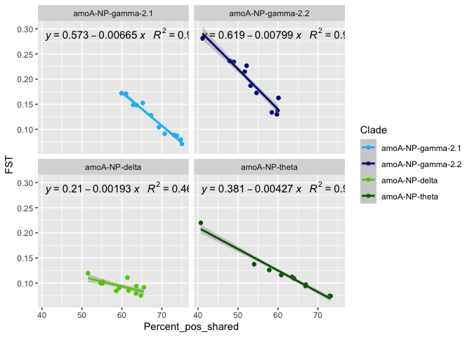
# correlation of FST distance with shared SNVs ?
correlation <- right_join(FST_A7_long_full, df_shared_SNVs_long_full, by = c("Sample_1" = "Sample_ID_1", "Sample_2" = "Sample_ID_2", "Sample1_horizon", "Sample2_horizon", "Sample1_core", "Sample2_core", "Clade"))

library(ggpmisc)

ggplot(correlation, aes(x = Percent_pos_shared, y = FST)) +
  geom_point(aes(color = Clade)) +
  geom_smooth(method = "lm", formula = y~x, aes(color = Clade)) +
  scale_color_manual(values = scale_amoA) +
  stat_poly_eq(formula = y~x,
               aes(label = paste(..eq.label.., ..rr.label.., sep = "~~~")),
               parse = TRUE, label.x = "left", label.y = "top", size = 4) +
  facet_wrap(~Clade)
correlation$Clade <- factor(correlation$Clade, levels = clade_list)
by(correlation, correlation$Clade, function(x) summary(lm(x$FST ~ x$Percent_pos_shared)))
## correlation$Clade: amoA-NP-gamma-2.1
##
## Call:
## lm(formula = x$FST ~ x$Percent_pos_shared)
##
## Residuals:
##        Min         1Q     Median         3Q        Max
## -0.0110725 -0.0037011  0.0002911  0.0041068  0.0136186
##
## Coefficients:
##                       Estimate Std. Error t value Pr(>|t|)
## (Intercept)           0.573025   0.017880   32.05   <2e-16 ***
## x$Percent_pos_shared -0.006654   0.000262  -25.40   <2e-16 ***
## ---
## Signif. codes:  0 '***' 0.001 '**' 0.01 '*' 0.05 '.' 0.1 ' ' 1
##
## Residual standard error: 0.006737 on 22 degrees of freedom
##   (2 observations deleted due to missingness)
## Multiple R-squared:  0.967,  Adjusted R-squared:  0.9655
## F-statistic: 645.1 on 1 and 22 DF,  p-value: < 2.2e-16
##
## ------------------------------------------------------------
## correlation$Clade: amoA-NP-gamma-2.2
##
## Call:
## lm(formula = x$FST ~ x$Percent_pos_shared)
##
## Residuals:
##       Min        1Q    Median        3Q       Max
## -0.018471 -0.009425 -0.002124  0.006434  0.023972
##
## Coefficients:
##                        Estimate Std. Error t value Pr(>|t|)
## (Intercept)           0.6192043  0.0257144   24.08  < 2e-16 ***
## x$Percent_pos_shared -0.0079872  0.0004825  -16.55 6.67e-14 ***
## ---
## Signif. codes:  0 '***' 0.001 '**' 0.01 '*' 0.05 '.' 0.1 ' ' 1
##
## Residual standard error: 0.01342 on 22 degrees of freedom
## Multiple R-squared:  0.9257, Adjusted R-squared:  0.9223
## F-statistic:   274 on 1 and 22 DF,  p-value: 6.666e-14
##
## ------------------------------------------------------------
## correlation$Clade: amoA-NP-delta
##
## Call:
## lm(formula = x$FST ~ x$Percent_pos_shared)
##
## Residuals:
##       Min        1Q    Median        3Q       Max
## -0.011706 -0.005952 -0.003735  0.007943  0.020100
##
## Coefficients:
##                        Estimate Std. Error t value Pr(>|t|)
## (Intercept)           0.2095681  0.0265097   7.905 7.19e-08 ***
## x$Percent_pos_shared -0.0019342  0.0004438  -4.359 0.000251 ***
## ---
## Signif. codes:  0 '***' 0.001 '**' 0.01 '*' 0.05 '.' 0.1 ' ' 1
##
## Residual standard error: 0.009515 on 22 degrees of freedom
##   (2 observations deleted due to missingness)
## Multiple R-squared:  0.4634, Adjusted R-squared:  0.439
## F-statistic:    19 on 1 and 22 DF,  p-value: 0.0002512
##
## ------------------------------------------------------------
## correlation$Clade: amoA-NP-theta
##
## Call:
## lm(formula = x$FST ~ x$Percent_pos_shared)
##
## Residuals:
##       Min        1Q    Median        3Q       Max
## -0.012961 -0.005409  0.001666  0.004604  0.012367
##
## Coefficients:
##                        Estimate Std. Error t value Pr(>|t|)
## (Intercept)           0.3813287  0.0112430   33.92  < 2e-16 ***
## x$Percent_pos_shared -0.0042708  0.0001791  -23.84 4.55e-15 ***
## ---
## Signif. codes:  0 '***' 0.001 '**' 0.01 '*' 0.05 '.' 0.1 ' ' 1
##
## Residual standard error: 0.007321 on 18 degrees of freedom
##   (2 observations deleted due to missingness)
## Multiple R-squared:  0.9693, Adjusted R-squared:  0.9676
## F-statistic: 568.4 on 1 and 18 DF,  p-value: 4.553e-15
# correlation of FST distance with shared SNVs with same consensus ?
ggplot(correlation, aes(x = Shared_same_consensus, y = FST)) +
  geom_point(aes(color = Clade)) +
  geom_smooth(method = "lm", formula = y~x, aes(color = Clade)) +
  scale_color_manual(values = scale_amoA) +
  stat_poly_eq(formula = y~x,
               aes(label = paste(..eq.label.., ..rr.label.., sep = "~~~")),
               parse = TRUE, label.x = "left", label.y = "top", size = 4) +
  facet_wrap(~Clade)
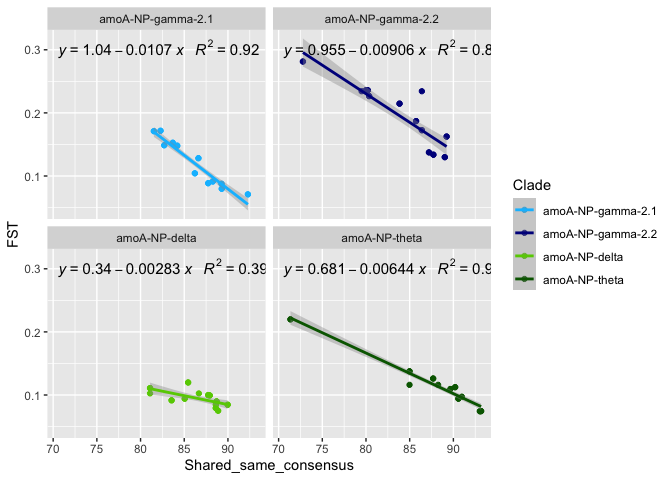
by(correlation, correlation$Clade, function(x) summary(lm(x$FST ~ x$Shared_same_consensus)))
## correlation$Clade: amoA-NP-gamma-2.1
##
## Call:
## lm(formula = x$FST ~ x$Shared_same_consensus)
##
## Residuals:
##        Min         1Q     Median         3Q        Max
## -0.0155554 -0.0074686  0.0007908  0.0075255  0.0157970
##
## Coefficients:
##                           Estimate Std. Error t value Pr(>|t|)
## (Intercept)              1.0386595  0.0580456   17.89 1.34e-14 ***
## x$Shared_same_consensus -0.0106576  0.0006731  -15.83 1.65e-13 ***
## ---
## Signif. codes:  0 '***' 0.001 '**' 0.01 '*' 0.05 '.' 0.1 ' ' 1
##
## Residual standard error: 0.01054 on 22 degrees of freedom
##   (2 observations deleted due to missingness)
## Multiple R-squared:  0.9193, Adjusted R-squared:  0.9157
## F-statistic: 250.7 on 1 and 22 DF,  p-value: 1.647e-13
##
## ------------------------------------------------------------
## correlation$Clade: amoA-NP-gamma-2.2
##
## Call:
## lm(formula = x$FST ~ x$Shared_same_consensus)
##
## Residuals:
##       Min        1Q    Median        3Q       Max
## -0.027568 -0.015417  0.000212  0.008632  0.061954
##
## Coefficients:
##                           Estimate Std. Error t value Pr(>|t|)
## (Intercept)              0.9551450  0.0752256   12.70 1.33e-11 ***
## x$Shared_same_consensus -0.0090608  0.0008964  -10.11 9.93e-10 ***
## ---
## Signif. codes:  0 '***' 0.001 '**' 0.01 '*' 0.05 '.' 0.1 ' ' 1
##
## Residual standard error: 0.02072 on 22 degrees of freedom
## Multiple R-squared:  0.8228, Adjusted R-squared:  0.8148
## F-statistic: 102.2 on 1 and 22 DF,  p-value: 9.931e-10
##
## ------------------------------------------------------------
## correlation$Clade: amoA-NP-delta
##
## Call:
## lm(formula = x$FST ~ x$Shared_same_consensus)
##
## Residuals:
##        Min         1Q     Median         3Q        Max
## -0.0127917 -0.0079835 -0.0002808  0.0084070  0.0221709
##
## Coefficients:
##                           Estimate Std. Error t value Pr(>|t|)
## (Intercept)              0.3397121  0.0651421   5.215 3.14e-05 ***
## x$Shared_same_consensus -0.0028328  0.0007516  -3.769  0.00106 **
## ---
## Signif. codes:  0 '***' 0.001 '**' 0.01 '*' 0.05 '.' 0.1 ' ' 1
##
## Residual standard error: 0.01013 on 22 degrees of freedom
##   (2 observations deleted due to missingness)
## Multiple R-squared:  0.3923, Adjusted R-squared:  0.3647
## F-statistic:  14.2 on 1 and 22 DF,  p-value: 0.001058
##
## ------------------------------------------------------------
## correlation$Clade: amoA-NP-theta
##
## Call:
## lm(formula = x$FST ~ x$Shared_same_consensus)
##
## Residuals:
##       Min        1Q    Median        3Q       Max
## -0.018334 -0.004999  0.001121  0.005064  0.011539
##
## Coefficients:
##                          Estimate Std. Error t value Pr(>|t|)
## (Intercept)              0.681407   0.025885   26.32 8.02e-16 ***
## x$Shared_same_consensus -0.006436   0.000294  -21.89 2.02e-14 ***
## ---
## Signif. codes:  0 '***' 0.001 '**' 0.01 '*' 0.05 '.' 0.1 ' ' 1
##
## Residual standard error: 0.007951 on 18 degrees of freedom
##   (2 observations deleted due to missingness)
## Multiple R-squared:  0.9638, Adjusted R-squared:  0.9618
## F-statistic: 479.1 on 1 and 18 DF,  p-value: 2.018e-14
library(FactoMineR)
library(factoextra)
library(missMDA)
library(Hmisc)
library(corrplot)

meta_corr <- correlation[correlation$Clade == "amoA-NP-delta", c(3,12:14)]
cor <- rcorr(as.matrix(meta_corr))
M <- cor$r
M
##                              FST Percent_pos_shared Shared_diff_consensus
## FST                    1.0000000         -0.6807253             0.6263568
## Percent_pos_shared    -0.6807253          1.0000000            -0.4748002
## Shared_diff_consensus  0.6263568         -0.4748002             1.0000000
## Shared_same_consensus -0.6263568          0.4748002            -1.0000000
##                       Shared_same_consensus
## FST                              -0.6263568
## Percent_pos_shared                0.4748002
## Shared_diff_consensus            -1.0000000
## Shared_same_consensus             1.0000000
# correlation of FST distance with SNV density for gamma-2.1
FST_dists <- read.table(here(paste0("NON_REDUNDANT_BINS/10_VAR_PROFILES/3_FST_SNV/FST_HAK_Bin_00079.txt")),
                          sep="\t", header=TRUE, row.names=1)
FST_A7 <-  FST_dists[rownames(FST_dists) %in% meta[meta$Site == "A7", "Sample_ID"], colnames(FST_dists) %in% meta[meta$Site == "A7", "Sample_ID"]]
df <- SNV_nb_df_gamma2.1[SNV_nb_df_gamma2.1$sample_id %in% colnames(FST_A7),]

NMDS.ord <- metaMDS(FST_A7)
## Run 0 stress 0.08365497
## Run 1 stress 0.06907032
## ... New best solution
## ... Procrustes: rmse 0.1598802  max resid 0.4199092
## Run 2 stress 0.09078543
## Run 3 stress 0.08009805
## Run 4 stress 0.07496952
## Run 5 stress 0.09402013
## Run 6 stress 0.0810684
## Run 7 stress 0.08365488
## Run 8 stress 0.06907039
## ... Procrustes: rmse 9.039759e-05  max resid 0.0001926964
## ... Similar to previous best
## Run 9 stress 0.08009819
## Run 10 stress 0.08113333
## Run 11 stress 0.07647398
## Run 12 stress 0.06907021
## ... New best solution
## ... Procrustes: rmse 0.0003866367  max resid 0.0008744305
## ... Similar to previous best
## Run 13 stress 0.08290755
## Run 14 stress 0.07787697
## Run 15 stress 0.08653765
## Run 16 stress 0.07496933
## Run 17 stress 0.08016378
## Run 18 stress 0.0829076
## Run 19 stress 0.08106859
## Run 20 stress 0.07334038
## *** Best solution repeated 1 times
#extract NMDS scores (x and y coordinates) for sites from newer versions of vegan package
data.scores = as.data.frame(scores(NMDS.ord))
data.scores$Sample_ID <- rownames(data.scores)

#add columns to data frame
data.scores <- left_join(data.scores, df, by = c("Sample_ID" = "sample_id"))

fit <- envfit(NMDS.ord~SNV_nb_kb,
              data = df, permutations = how(nperm = 999), display = "sites", na.rm=T)
fit
##
## ***VECTORS
##
##              NMDS1    NMDS2    r2 Pr(>r)
## SNV_nb_kb  0.91259 -0.40887 0.136  0.536
## Permutation: free
## Number of permutations: 999
# correlation of FST distance with SNV density for gamma-2.2
FST_dists <- read.table(here(paste0("NON_REDUNDANT_BINS/10_VAR_PROFILES/3_FST_SNV/FST_HAS_Bin_00039.txt")),
                          sep="\t", header=TRUE, row.names=1)
FST_A7 <-  FST_dists[rownames(FST_dists) %in% meta[meta$Site == "A7", "Sample_ID"], colnames(FST_dists) %in% meta[meta$Site == "A7", "Sample_ID"]]
df <- SNV_nb_df_gamma2.2[SNV_nb_df_gamma2.2$sample_id %in% colnames(FST_A7),]

NMDS.ord <- metaMDS(FST_A7)
## Run 0 stress 9.95841e-05
## Run 1 stress 9.49493e-05
## ... New best solution
## ... Procrustes: rmse 0.0002030363  max resid 0.0006177676
## ... Similar to previous best
## Run 2 stress 9.562463e-05
## ... Procrustes: rmse 0.0002218685  max resid 0.0004055615
## ... Similar to previous best
## Run 3 stress 9.781605e-05
## ... Procrustes: rmse 0.0001926896  max resid 0.0006423536
## ... Similar to previous best
## Run 4 stress 9.704736e-05
## ... Procrustes: rmse 0.000266606  max resid 0.0007409221
## ... Similar to previous best
## Run 5 stress 9.949407e-05
## ... Procrustes: rmse 0.0001082743  max resid 0.0001996324
## ... Similar to previous best
## Run 6 stress 9.944541e-05
## ... Procrustes: rmse 0.0002687373  max resid 0.0007351771
## ... Similar to previous best
## Run 7 stress 9.88484e-05
## ... Procrustes: rmse 0.0001439507  max resid 0.0004490408
## ... Similar to previous best
## Run 8 stress 9.886196e-05
## ... Procrustes: rmse 0.0002309498  max resid 0.0004214689
## ... Similar to previous best
## Run 9 stress 9.527712e-05
## ... Procrustes: rmse 0.0001638684  max resid 0.0003230688
## ... Similar to previous best
## Run 10 stress 9.961176e-05
## ... Procrustes: rmse 5.141929e-05  max resid 9.42717e-05
## ... Similar to previous best
## Run 11 stress 9.511255e-05
## ... Procrustes: rmse 0.000114039  max resid 0.0003161831
## ... Similar to previous best
## Run 12 stress 0.0001735649
## ... Procrustes: rmse 0.0004693395  max resid 0.001054541
## ... Similar to previous best
## Run 13 stress 9.602146e-05
## ... Procrustes: rmse 4.958822e-05  max resid 9.642378e-05
## ... Similar to previous best
## Run 14 stress 9.488322e-05
## ... New best solution
## ... Procrustes: rmse 0.0001565926  max resid 0.0004186611
## ... Similar to previous best
## Run 15 stress 9.909481e-05
## ... Procrustes: rmse 0.0001885055  max resid 0.0003925116
## ... Similar to previous best
## Run 16 stress 9.883599e-05
## ... Procrustes: rmse 9.350829e-05  max resid 0.0002251627
## ... Similar to previous best
## Run 17 stress 9.901697e-05
## ... Procrustes: rmse 0.0002069781  max resid 0.0005968641
## ... Similar to previous best
## Run 18 stress 9.806575e-05
## ... Procrustes: rmse 4.558251e-05  max resid 0.0001105049
## ... Similar to previous best
## Run 19 stress 9.959024e-05
## ... Procrustes: rmse 0.0002085257  max resid 0.000600014
## ... Similar to previous best
## Run 20 stress 9.89e-05
## ... Procrustes: rmse 0.0002067374  max resid 0.0005960607
## ... Similar to previous best
## *** Best solution repeated 7 times
#extract NMDS scores (x and y coordinates) for sites from newer versions of vegan package
data.scores = as.data.frame(scores(NMDS.ord))
data.scores$Sample_ID <- rownames(data.scores)

#add columns to data frame
data.scores <- left_join(data.scores, df, by = c("Sample_ID" = "sample_id"))

fit <- envfit(NMDS.ord~SNV_nb_kb,
              data = df, permutations = how(nperm = 999), display = "sites", na.rm=T)
fit
##
## ***VECTORS
##
##                 NMDS1       NMDS2     r2 Pr(>r)
## SNV_nb_kb -0.00096301 -1.00000000 0.8533  0.001 ***
## ---
## Signif. codes:  0 '***' 0.001 '**' 0.01 '*' 0.05 '.' 0.1 ' ' 1
## Permutation: free
## Number of permutations: 999
# correlation of FST distance with SNV density for delta
FST_dists <- read.table(here(paste0("NON_REDUNDANT_BINS/10_VAR_PROFILES/3_FST_SNV/FST_H3T_Bin_00024.txt")),
                          sep="\t", header=TRUE, row.names=1)
FST_A7 <-  FST_dists[rownames(FST_dists) %in% meta[meta$Site == "A7", "Sample_ID"], colnames(FST_dists) %in% meta[meta$Site == "A7", "Sample_ID"]]
df <- SNV_nb_df_delta[SNV_nb_df_delta$sample_id %in% colnames(FST_A7),]

NMDS.ord <- metaMDS(FST_A7)
## Run 0 stress 0.08461712
## Run 1 stress 0.08579292
## Run 2 stress 0.0870155
## Run 3 stress 0.08591061
## Run 4 stress 0.08520436
## Run 5 stress 0.08193131
## ... New best solution
## ... Procrustes: rmse 0.1244338  max resid 0.3309266
## Run 6 stress 0.08377979
## Run 7 stress 0.0859105
## Run 8 stress 0.090557
## Run 9 stress 0.08683652
## Run 10 stress 0.08377972
## Run 11 stress 0.118212
## Run 12 stress 0.08498831
## Run 13 stress 0.0849884
## Run 14 stress 0.08610486
## Run 15 stress 0.08193131
## ... Procrustes: rmse 1.354163e-05  max resid 3.301479e-05
## ... Similar to previous best
## Run 16 stress 0.0910273
## Run 17 stress 0.1139632
## Run 18 stress 0.0807348
## ... New best solution
## ... Procrustes: rmse 0.04141776  max resid 0.1255461
## Run 19 stress 0.08701547
## Run 20 stress 0.08498828
## *** Best solution was not repeated -- monoMDS stopping criteria:
##     20: stress ratio > sratmax
#extract NMDS scores (x and y coordinates) for sites from newer versions of vegan package
data.scores = as.data.frame(scores(NMDS.ord))
data.scores$Sample_ID <- rownames(data.scores)

#add columns to data frame
data.scores <- left_join(data.scores, df, by = c("Sample_ID" = "sample_id"))

fit <- envfit(NMDS.ord~SNV_nb_kb,
              data = df, permutations = how(nperm = 999), display = "sites", na.rm=T)
fit
##
## ***VECTORS
##
##               NMDS1     NMDS2     r2 Pr(>r)
## SNV_nb_kb -0.999680  0.025399 0.9288  0.001 ***
## ---
## Signif. codes:  0 '***' 0.001 '**' 0.01 '*' 0.05 '.' 0.1 ' ' 1
## Permutation: free
## Number of permutations: 999
# correlation of FST distance with SNV density for theta
FST_dists <- read.table(here(paste0("NON_REDUNDANT_BINS/10_VAR_PROFILES/3_FST_SNV/FST_A9S_Bin_00032.txt")),
                          sep="\t", header=TRUE, row.names=1)
FST_A7 <-  FST_dists[rownames(FST_dists) %in% meta[meta$Site == "A7", "Sample_ID"], colnames(FST_dists) %in% meta[meta$Site == "A7", "Sample_ID"]]
df <- SNV_nb_df_theta[SNV_nb_df_theta$sample_id %in% colnames(FST_A7),]

NMDS.ord <- metaMDS(FST_A7)
## Run 0 stress 0.05919792
## Run 1 stress 0.06715679
## Run 2 stress 0.06398926
## Run 3 stress 0.07525733
## Run 4 stress 0.05770491
## ... New best solution
## ... Procrustes: rmse 0.06207233  max resid 0.2103438
## Run 5 stress 0.06292897
## Run 6 stress 0.3432087
## Run 7 stress 0.06299657
## Run 8 stress 0.05793447
## ... Procrustes: rmse 0.05075985  max resid 0.1031865
## Run 9 stress 0.05643648
## ... New best solution
## ... Procrustes: rmse 0.04239036  max resid 0.1007591
## Run 10 stress 0.06715694
## Run 11 stress 0.06299446
## Run 12 stress 0.06397693
## Run 13 stress 0.3532053
## Run 14 stress 0.05643664
## ... Procrustes: rmse 0.0001170094  max resid 0.000278915
## ... Similar to previous best
## Run 15 stress 0.0694838
## Run 16 stress 0.06887212
## Run 17 stress 0.06896668
## Run 18 stress 0.06715695
## Run 19 stress 0.06292794
## Run 20 stress 0.06948601
## *** Best solution repeated 1 times
#extract NMDS scores (x and y coordinates) for sites from newer versions of vegan package
data.scores = as.data.frame(scores(NMDS.ord))
data.scores$Sample_ID <- rownames(data.scores)

#add columns to data frame
data.scores <- left_join(data.scores, df, by = c("Sample_ID" = "sample_id"))

fit <- envfit(NMDS.ord~SNV_nb_kb,
              data = df, permutations = how(nperm = 999), display = "sites", na.rm=T)
fit
##
## ***VECTORS
##
##             NMDS1   NMDS2     r2 Pr(>r)
## SNV_nb_kb 0.46073 0.88754 0.1188  0.477
## Permutation: free
## Number of permutations: 999
Figure S1: sample map extracted from Glud et al., 2021
Figure S2: amoA phylogenetic tree
tree <- treeio::read.jplace(here("09_amoA_tree/epa_result_amoA_int_ext.jplace"))
tree@placements <- get.placements(tree, by="best")
placement_MAGs <- tree@placements

# to simplify the comparison, I extracted the placement info for amoA genes on a co-assembly only tree
placement <- read.table(here("09_amoA_tree/Placement_coA_amoA.txt"), header = TRUE)
coassembly_amoA <- unique(placement$node)

int_MAG_amoA <- pull(unique(placement_MAGs[grep("_Bin_", placement_MAGs$name), "node"]))
ext_MAG_amoA <- pull(unique(placement_MAGs[-grep("_Bin_", placement_MAGs$name), "node"]))
# I need the node number to collapse, color, etc
## getting node number, using a tibble + common ancestor
tb <- as_tibble(tree)
MRCA(tb, 742, 1186) # NS Nitrososphaerales
## # A tibble: 1 × 5
##   parent  node branch.length label nplace
##    <int> <int>         <dbl> <chr>  <dbl>
## 1   1192  1933        0.0611 <NA>       0
MRCA(tb, 625, 741) # NT Nitrosotaleales, NT NP Incertae sedis not included (621 to 624)
## # A tibble: 1 × 5
##   parent  node branch.length label nplace
##    <int> <int>         <dbl> <chr>  <dbl>
## 1   1193  1817        0.0924 <NA>       0
MRCA(tb, 1, 620) # NP Nitropumilales
## # A tibble: 1 × 5
##   parent  node branch.length label nplace
##    <int> <int>         <dbl> <chr>  <dbl>
## 1   1194  1195        0.0473 <NA>       0
MRCA(tb, 1187, 1190) # NC
## # A tibble: 1 × 5
##   parent  node branch.length label nplace
##    <int> <int>         <dbl> <chr>  <dbl>
## 1   1191  2377        0.0857 <NA>       0
# annotate the full tree with the clades
x <- ggtree(tree, layout='circular') +
  geom_cladelabel(1817, "Nitrosotalea", barsize=1, fontsize=4, offset.text=0.1, angle=60, hjust=0.5) +
  geom_cladelabel(1933, "Nitrososphaeraceae", barsize=1, fontsize=4, offset.text=0.1, angle=-30, hjust=0.3) +
  #geom_cladelabel(1195, "Nitrosopumilales", barsize=1, fontsize=4, offset.text=0.1, angle=0, hjust=0.3, offset = 0.2) +
  geom_cladelabel(2377, "Nitrosocaldaceae", fontsize=4, offset.text=0.5, angle=0)


## getting node number, using a tibble + common ancestor
MRCA(tb, 1, 207) # Gamma - NP
## # A tibble: 1 × 5
##   parent  node branch.length label nplace
##    <int> <int>         <dbl> <chr>  <dbl>
## 1   1199  1200        0.0289 <NA>       0
MRCA(tb, 208, 312) # Alpha - NP
## # A tibble: 1 × 5
##   parent  node branch.length label nplace
##    <int> <int>         <dbl> <chr>  <dbl>
## 1   1406  1407         0.105 <NA>       0
MRCA(tb, 313, 322) # Beta - NP
## # A tibble: 1 × 5
##   parent  node branch.length label nplace
##    <int> <int>         <dbl> <chr>  <dbl>
## 1   1406  1511        0.0921 <NA>       0
MRCA(tb, 510, 620) # Delta - NP
## # A tibble: 1 × 5
##   parent  node branch.length label nplace
##    <int> <int>         <dbl> <chr>  <dbl>
## 1   1195  1704        0.0362 <NA>       0
MRCA(tb, 341, 414) # Theta - NP
## # A tibble: 1 × 5
##   parent  node branch.length label nplace
##    <int> <int>         <dbl> <chr>  <dbl>
## 1   1197  1537        0.0143 <NA>       0
MRCA(tb, 415, 475) # Eta - NP
## # A tibble: 1 × 5
##   parent  node branch.length label nplace
##    <int> <int>         <dbl> <chr>  <dbl>
## 1   1610  1611        0.0356 <NA>       0
MRCA(tb, 476, 509) # Epsilon - NP
## # A tibble: 1 × 5
##   parent  node branch.length label nplace
##    <int> <int>         <dbl> <chr>  <dbl>
## 1   1610  1671        0.0363 <NA>       0
MRCA(tb, 323, 340) # Zeta - NP
## # A tibble: 1 × 5
##   parent  node branch.length label nplace
##    <int> <int>         <dbl> <chr>  <dbl>
## 1   1198  1520        0.0353 <NA>       0
MRCA(tb, 621, 624) # NT/NP Incertae Sedis
## # A tibble: 1 × 5
##   parent  node branch.length label nplace
##    <int> <int>         <dbl> <chr>  <dbl>
## 1   1194  1814        0.0412 <NA>       0
MRCA(tb, 1, 96) # gamma 2.2
## # A tibble: 1 × 5
##   parent  node branch.length label nplace
##    <int> <int>         <dbl> <chr>  <dbl>
## 1   1201  1202        0.0210 <NA>       0
MRCA(tb, 97, 187) # gamma 2.1
## # A tibble: 1 × 5
##   parent  node branch.length label nplace
##    <int> <int>         <dbl> <chr>  <dbl>
## 1   1201  1297        0.0139 <NA>       0
MRCA(tb, 203, 205) # gamma 3
## # A tibble: 1 × 5
##   parent  node branch.length label nplace
##    <int> <int>         <dbl> <chr>  <dbl>
## 1   1402  1403        0.0223 <NA>       0
MRCA(tb, 625, 720) # NT alpha
## # A tibble: 1 × 5
##   parent  node branch.length label nplace
##    <int> <int>         <dbl> <chr>  <dbl>
## 1   1818  1819        0.0559 <NA>       0
# adding clades
p <- x + geom_cladelabel(1297, "NP-Gamma-2.1", barsize=1, fontsize=4, offset = 0.1, hjust = -0.3) +
  geom_hilight(node=1297, fill="deepskyblue", alpha=0.2, extend = 0.1) + # gamma 2.1
  geom_cladelabel(1202, "NP-Gamma-2.2", barsize=1, fontsize=4, offset = 0.1, hjust = -0.3) +
  geom_hilight(node=1202, fill="darkblue", alpha=0.2, extend = 0.1) +# gamma 2.2
  geom_cladelabel(1403, "NP-Gamma-3", barsize=1, fontsize=4, offset.text=0.5, angle = -60) +
  geom_hilight(node=1403, fill="cyan", alpha=0.5, extend = 0.5) + # gamma 3
  geom_cladelabel(1407, "NP-Alpha", barsize=1, fontsize=4, hjust=0.5, offset.text=0.1) + geom_hilight(node=1407, fill="gold", alpha=0.2) +
  geom_cladelabel(1511, "NP-Beta", barsize=1, fontsize=4, offset.text=0.5, hjust=0.5, angle = 90) +
  geom_cladelabel(1704, "NP-Delta", barsize=1, fontsize=4, offset.text=0.3) + geom_hilight(node=1704, fill="chartreuse3", alpha=0.2) +
  geom_cladelabel(1537, "NP-Theta", barsize=1, fontsize=4, hjust=1) + geom_hilight(node=1537, fill="darkgreen", alpha=0.2) +
  geom_cladelabel(1611, "NP-Eta", barsize=1, fontsize=4, hjust=1) +
  geom_cladelabel(1671, "NP-Epsilon", barsize=1, fontsize=4, hjust=1) +
  geom_cladelabel(1520, "NP-Zeta", barsize=1, fontsize=4, offset.text=0.5, hjust=0.5, angle = 90) +
  geom_cladelabel(1814, "NP-Iota", barsize=1, fontsize=4, offset.text=0.4, hjust=1) + geom_hilight(node=1814, fill="bisque", alpha=0.6, extend = 0.4) +
  geom_hilight(node=2377, fill="coral1", alpha=0.5, extend = 0.5) # NC_alpha

# add the placement of my MAG amoA
tb[tb$nplace != 0, ] %>% print(n = Inf)
## # A tibble: 26 × 5
##    parent  node branch.length label                                       nplace
##     <int> <int>         <dbl> <chr>                                        <dbl>
##  1   1254    48       0.0348  NP-Gamma-2.2.2.Incertae_sedis_OTU2__KJ5097…      3
##  2   1315    99       0.0407  NP-Gamma-2.1.3.2.2.2_OTU3__KJ509742              1
##  3   1320   107       0.0303  NP-Gamma-2.1.3.2.2.2_OTU12__KJ509744             1
##  4   1384   180       0.0211  NP-Gamma-2.1.2_OTU2__AB583399                    1
##  5   1384   181       0.0312  NP-Gamma-2.1.2_OTU1__AB704000                    1
##  6   1381   182       0.0217  NP-Gamma-2.1.2_OTU5__EU427937                    1
##  7   1547   347       0.0284  NP-Theta-2.2.2.1_OTU7__KF178200                  1
##  8   1545   349       0.0130  NP-Theta-2.2.2.1_OTU9__KF178070                  1
##  9   1542   354       0.0339  NP-Theta-2.2_OTU1__AB827257                      4
## 10   1556   355       0.0205  NP-Theta-2.2.1_OTU1__JF924607                    1
## 11   1574   374       0.0241  NP-Theta-2.1.2_OTU3__AB827250                    1
## 12   1720   513       0.0343  NP-Delta-2.3.1.1_OTU5__JX537606                  1
## 13   1752   555       0.0106  NP-Delta-2.2.2_OTU2__EU885624                    1
## 14   1790   584       0.0196  NP-Delta-1.1.1_OTU5__KF178057                    2
## 15   1816   624       0.0172  NT_NP-Incertae_sedis-2_OTU2__FJ888623            1
## 16   2377  1190       0.369   NC_OTU1__JX311792                                1
## 17   1379  1380       0.0106  <NA>                                             2
## 18   1380  1381       0.0210  <NA>                                             1
## 19   1381  1382       0.0298  <NA>                                             2
## 20   1382  1383       0.0160  <NA>                                             1
## 21   1382  1384       0.0154  <NA>                                             1
## 22   1476  1477       0.0143  <NA>                                             1
## 23   1550  1551       0.00234 <NA>                                             1
## 24   1551  1552       0.0240  <NA>                                             1
## 25   1681  1687       0.00833 <NA>                                             1
## 26   1720  1721       0.0178  <NA>                                             1
q <- p +
  ## CoAssembly
  geom_point2(aes(subset=(node %in% coassembly_amoA)), shape=24, size=3, fill='yellow') +
  ## MAGs
  geom_point2(aes(subset=(node %in% int_MAG_amoA)), shape=24, size=3, fill='red')

#svg(here::here("Export_figures/amoA_Alves_tree_internal.svg"), width=12, height=18)
### Placement of amoA genes from internal MAGs and co-assembly
q
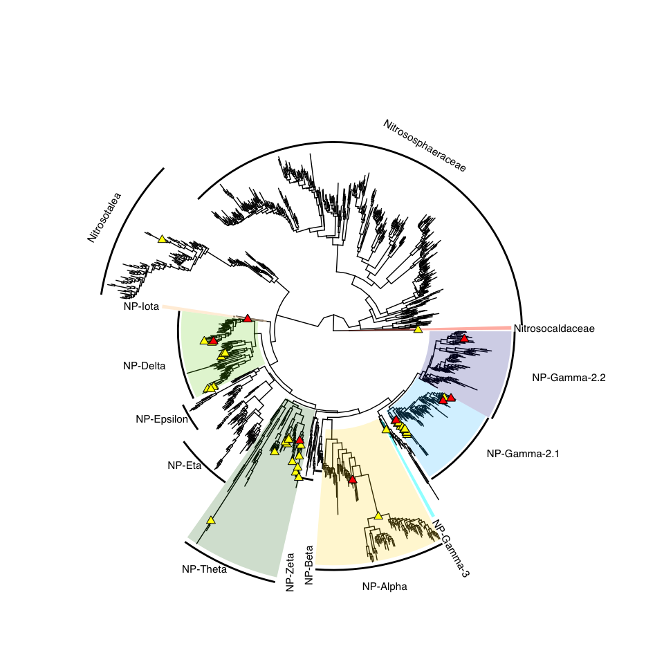
#dev.off()

q <- p +
  ## REFs
  geom_point2(aes(subset=(node %in% ext_MAG_amoA)), shape=23, size=3, fill='seagreen')

#svg(here::here("Export_figures/amoA_Alves_tree_external.svg"), width=12, height=18)
### Placement of amoA genes from external MAGs
q
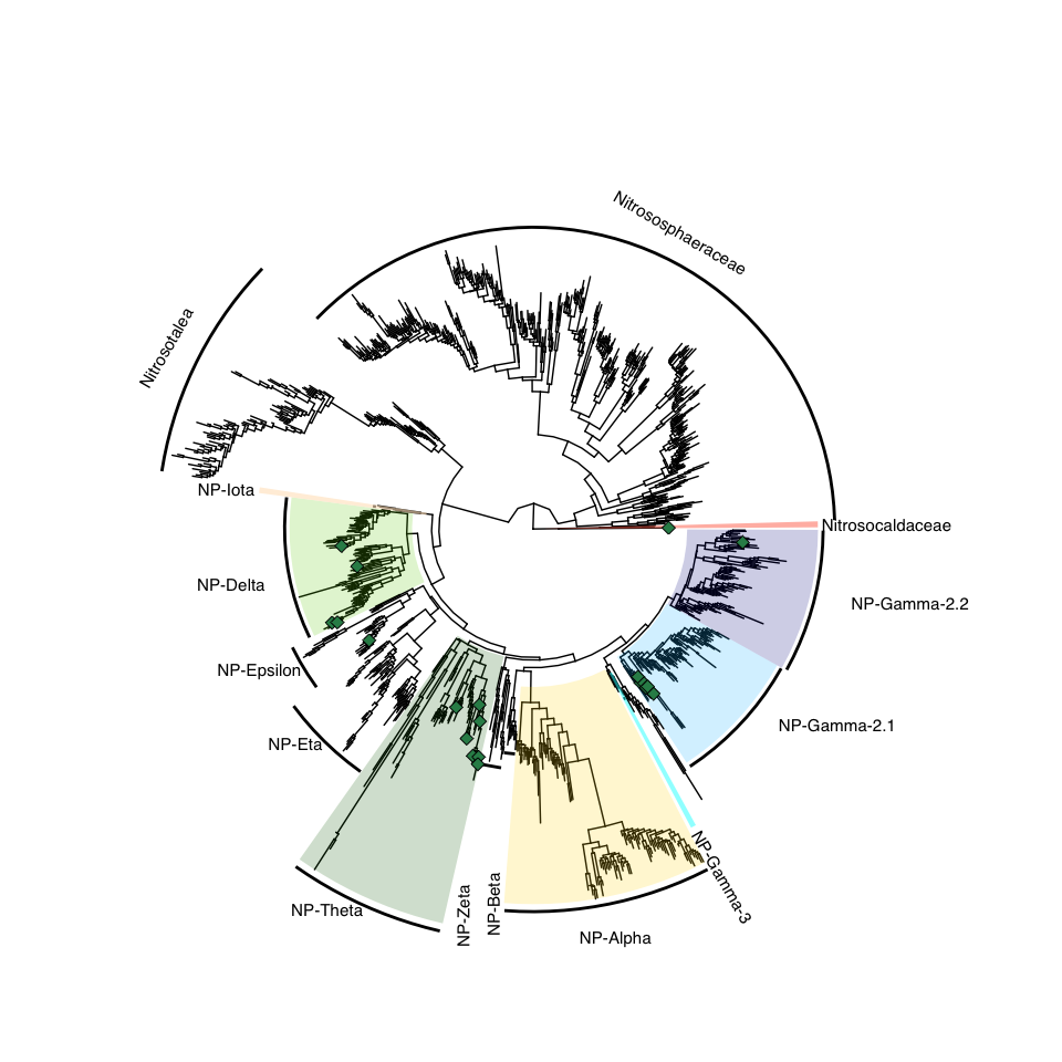
#dev.off()
Figure S3: FST-based trees for other gamma-2.1
# H3T_Bin_00167: gamma-2.1, SNV
H3T_Bin_00167_FST <- treeio::read.tree(here("NON_REDUNDANT_BINS/10_VAR_PROFILES/3_FST_SNV/FST_H3T_Bin_00167.newick"))
FST_simple <- full_join(H3T_Bin_00167_FST, meta[meta$Sample_ID %in% H3T_Bin_00167_FST$tip.label,],
                        by = c("label" = "Sample_ID"))

x_simple <- ggtree(FST_simple, branch.length="none") +
  geom_tiplab(aes(label=Simple_labels), size=5, offset=0.1)

#svg(here::here("Export_figures/Fig_S3_H3T167_SNV_FST.svg"), width=10, height=12)
x_simple + xlim(0,100)
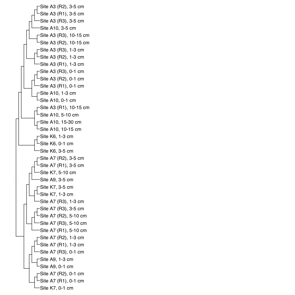
#dev.off()
# AK7_Bin_00137: gamma-2.1, SNV
AK7_Bin_00137_FST <- treeio::read.tree(here("NON_REDUNDANT_BINS/10_VAR_PROFILES/3_FST_SNV/FST_AK7_Bin_00137.newick"))
FST_simple <- full_join(AK7_Bin_00137_FST, meta[meta$Sample_ID %in% AK7_Bin_00137_FST$tip.label,],
                        by = c("label" = "Sample_ID"))

x_simple <- ggtree(FST_simple, branch.length="none") +
  geom_tiplab(aes(label=Simple_labels), size=5, offset=0.1)

#svg(here::here("Export_figures/Fig_S3_AK7137_SNV_FST.svg"), width=10, height=12)
x_simple + xlim(0,100)
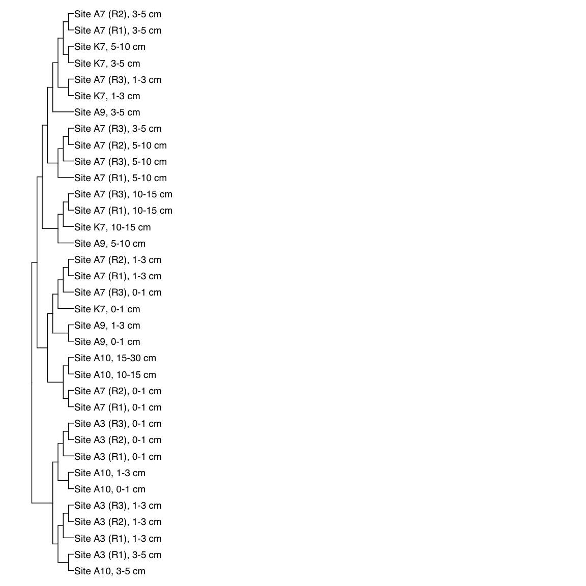
#dev.off()
# H3D_Bin_00215: gamma-2.1, SNV
H3D_Bin_00215_FST <- treeio::read.tree(here("NON_REDUNDANT_BINS/10_VAR_PROFILES/3_FST_SNV/FST_H3D_Bin_00215.newick"))
FST_simple <- full_join(H3D_Bin_00215_FST, meta[meta$Sample_ID %in% H3D_Bin_00215_FST$tip.label,],
                        by = c("label" = "Sample_ID"))

x_simple <- ggtree(FST_simple, branch.length="none") +
  geom_tiplab(aes(label=Simple_labels), size=5, offset=0.1)

#svg(here::here("Export_figures/Fig_S3_H3D215_SNV_FST.svg"), width=10, height=12)
x_simple + xlim(0,100)
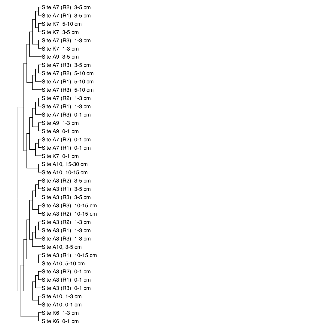
#dev.off()
# HKT_Bin_00027: gamma-2.1, SNV
HKT_Bin_00027_FST <- treeio::read.tree(here("NON_REDUNDANT_BINS/10_VAR_PROFILES/3_FST_SNV/FST_HKT_Bin_00027.newick"))
FST_simple <- full_join(HKT_Bin_00027_FST, meta[meta$Sample_ID %in% HKT_Bin_00027_FST$tip.label,],
                        by = c("label" = "Sample_ID"))

x_simple <- ggtree(FST_simple, branch.length="none") +
  geom_tiplab(aes(label=Simple_labels), size=5, offset=0.1)

#svg(here::here("Export_figures/Fig_S3_HKT27_SNV_FST.svg"), width=10, height=12)
x_simple + xlim(0,100)
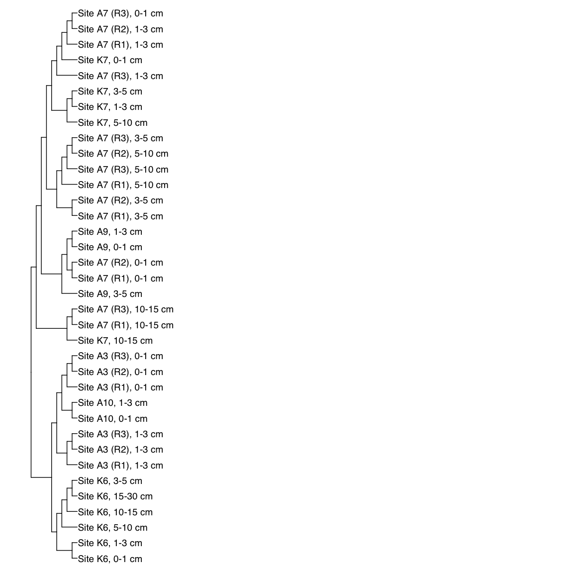
#dev.off()
# HKT_Bin_00076: gamma-2.1, SNV
HKT_Bin_00076_FST <- treeio::read.tree(here("NON_REDUNDANT_BINS/10_VAR_PROFILES/3_FST_SNV/FST_HKT_Bin_00076.newick"))
FST_simple <- full_join(HKT_Bin_00076_FST, meta[meta$Sample_ID %in% HKT_Bin_00076_FST$tip.label,],
                        by = c("label" = "Sample_ID"))

x_simple <- ggtree(FST_simple, branch.length="none") +
  geom_tiplab(aes(label=Simple_labels), size=5, offset=0.1)

#svg(here::here("Export_figures/Fig_S3_HKT76_SNV_FST.svg"), width=10, height=12)
x_simple + xlim(0,100)
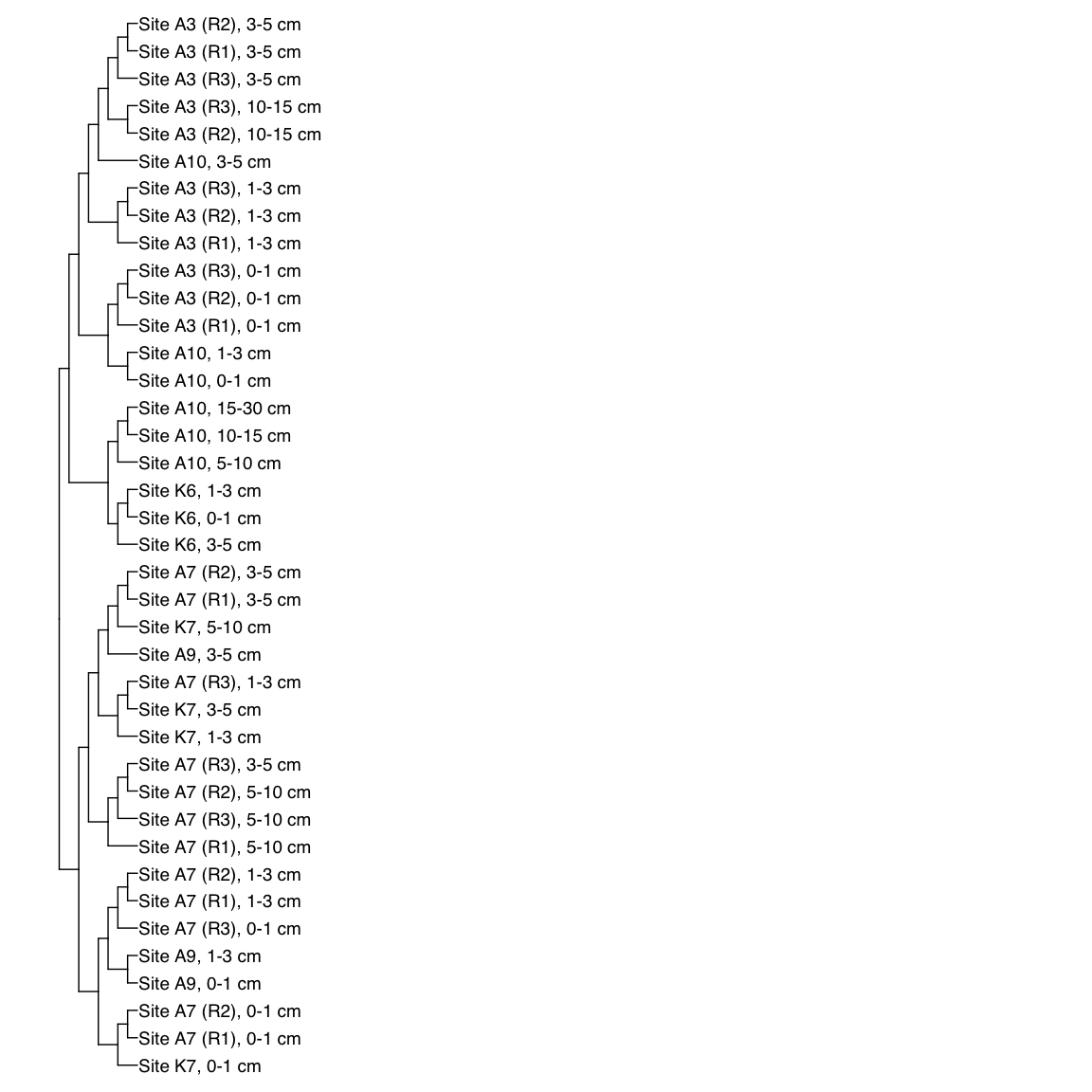
#dev.off()
# HKT_Bin_00075: gamma-2.1, SNV
HKT_Bin_00075_FST <- treeio::read.tree(here("NON_REDUNDANT_BINS/10_VAR_PROFILES/3_FST_SNV/FST_HKT_Bin_00075.newick"))
FST_simple <- full_join(HKT_Bin_00075_FST, meta[meta$Sample_ID %in% HKT_Bin_00075_FST$tip.label,],
                        by = c("label" = "Sample_ID"))

x_simple <- ggtree(FST_simple, branch.length="none") +
  geom_tiplab(aes(label=Simple_labels), size=5, offset=0.1)

#svg(here::here("Export_figures/Fig_S3_HKT75_SNV_FST.svg"), width=10, height=12)
x_simple + xlim(0,100)
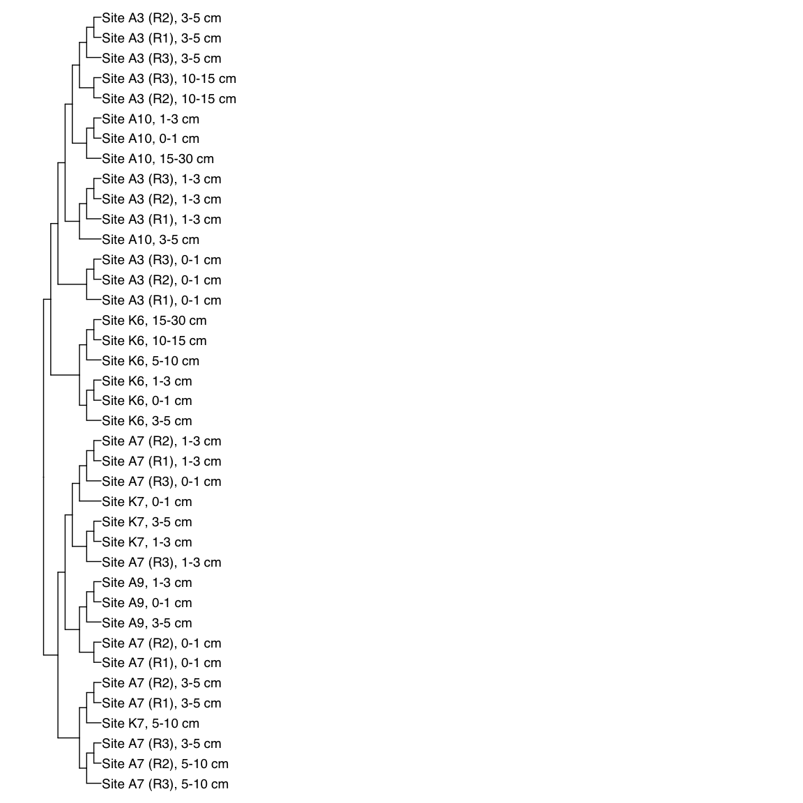
#dev.off()
Figure S4: FST-based trees for other gamma-2.2
# HKT_Bin_00022: gamma-2.2, SNV
HKT_Bin_00022_FST <- treeio::read.tree(here("NON_REDUNDANT_BINS/10_VAR_PROFILES/3_FST_SNV/FST_HKT_Bin_00022.newick"))
FST_simple <- full_join(HKT_Bin_00022_FST, meta[meta$Sample_ID %in% HKT_Bin_00022_FST$tip.label,],
                        by = c("label" = "Sample_ID"))

x_simple <- ggtree(FST_simple, branch.length="none") +
  geom_tiplab(aes(label=Simple_labels), size=5, offset=0.1)

#svg(here::here("Export_figures/Fig_S4_HKT22_SNV_FST.svg"), width=10, height=12)
x_simple + xlim(0,100)
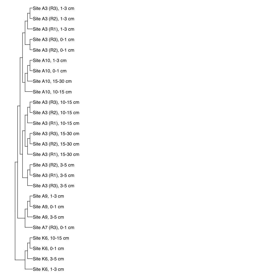
#dev.off()
Figure S5: FST-based trees for other delta
# A7D_Bin_00065: gamma-2.2, SNV
A7D_Bin_00065_FST <- treeio::read.tree(here("NON_REDUNDANT_BINS/10_VAR_PROFILES/3_FST_SNV/FST_A7D_Bin_00065.newick"))
FST_simple <- full_join(A7D_Bin_00065_FST, meta[meta$Sample_ID %in% A7D_Bin_00065_FST$tip.label,],
                        by = c("label" = "Sample_ID"))

x_simple <- ggtree(FST_simple, branch.length="none") +
  geom_tiplab(aes(label=Simple_labels), size=5, offset=0.1)

#svg(here::here("Export_figures/Fig_S5_A7D65_SNV_FST.svg"), width=10, height=12)
x_simple + xlim(0,100)
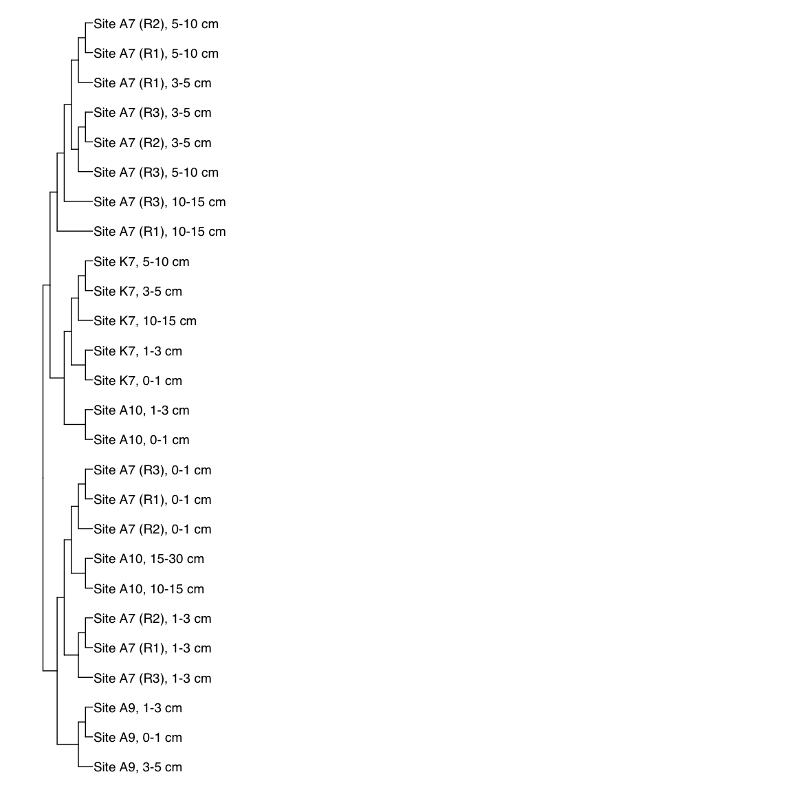
#dev.off()
# A9S_Bin_00058: gamma-2.2, SNV
A9S_Bin_00058_FST <- treeio::read.tree(here("NON_REDUNDANT_BINS/10_VAR_PROFILES/3_FST_SNV/FST_A9S_Bin_00058.newick"))
FST_simple <- full_join(A9S_Bin_00058_FST, meta[meta$Sample_ID %in% A9S_Bin_00058_FST$tip.label,],
                        by = c("label" = "Sample_ID"))

x_simple <- ggtree(FST_simple, branch.length="none") +
  geom_tiplab(aes(label=Simple_labels), size=5, offset=0.1)

#(here::here("Export_figures/Fig_S5_A9S58_SNV_FST.svg"), width=10, height=12)
x_simple + xlim(0,100)
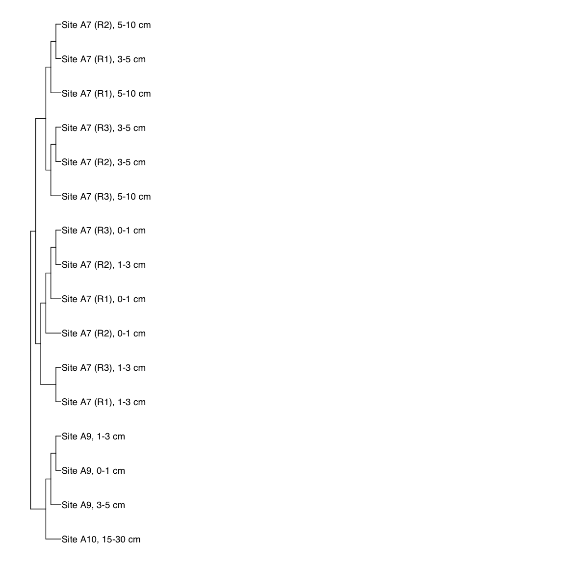
#dev.off()
# A7D_Bin_00052: gamma-2.2, SNV
A7D_Bin_00052_FST <- treeio::read.tree(here("NON_REDUNDANT_BINS/10_VAR_PROFILES/3_FST_SNV/FST_A7D_Bin_00052.newick"))
FST_simple <- full_join(A7D_Bin_00052_FST, meta[meta$Sample_ID %in% A7D_Bin_00052_FST$tip.label,],
by = c("label" = "Sample_ID"))
x_simple <- ggtree(FST_simple, branch.length="none") +
geom_tiplab(aes(label=Simple_labels), size=5, offset=0.1)
#svg(here::here("Export_figures/Fig_S5_A7D52_SNV_FST.svg"), width=10, height=12)
x_simple + xlim(0,100)
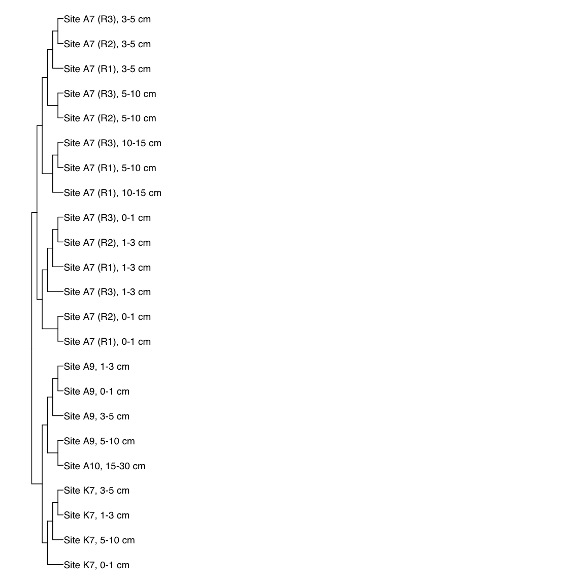
#dev.off()
# AK7_Bin_00037: gamma-2.2, SNV
AK7_Bin_00037_FST <- treeio::read.tree(here("NON_REDUNDANT_BINS/10_VAR_PROFILES/3_FST_SNV/FST_AK7_Bin_00037.newick"))
FST_simple <- full_join(AK7_Bin_00037_FST, meta[meta$Sample_ID %in% AK7_Bin_00037_FST$tip.label,],
by = c("label" = "Sample_ID"))
x_simple <- ggtree(FST_simple, branch.length="none") +
geom_tiplab(aes(label=Simple_labels), size=5, offset=0.1)
#svg(here::here("Export_figures/Fig_S5_AK737_SNV_FST.svg"), width=10, height=12)
x_simple + xlim(0,100)
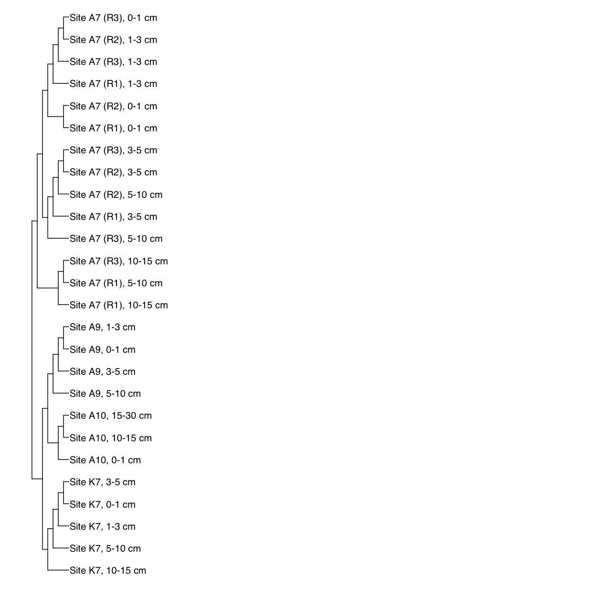
#dev.off()
# AK7_Bin_00136: gamma-2.2, SNV
AK7_Bin_00136_FST <- treeio::read.tree(here("NON_REDUNDANT_BINS/10_VAR_PROFILES/3_FST_SNV/FST_AK7_Bin_00136.newick"))
FST_simple <- full_join(AK7_Bin_00136_FST, meta[meta$Sample_ID %in% AK7_Bin_00136_FST$tip.label,],
by = c("label" = "Sample_ID"))
x_simple <- ggtree(FST_simple, branch.length="none") +
geom_tiplab(aes(label=Simple_labels), size=5, offset=0.1)
#svg(here::here("Export_figures/Fig_S5_AK7136_SNV_FST.svg"), width=10, height=12)
x_simple + xlim(0,100)
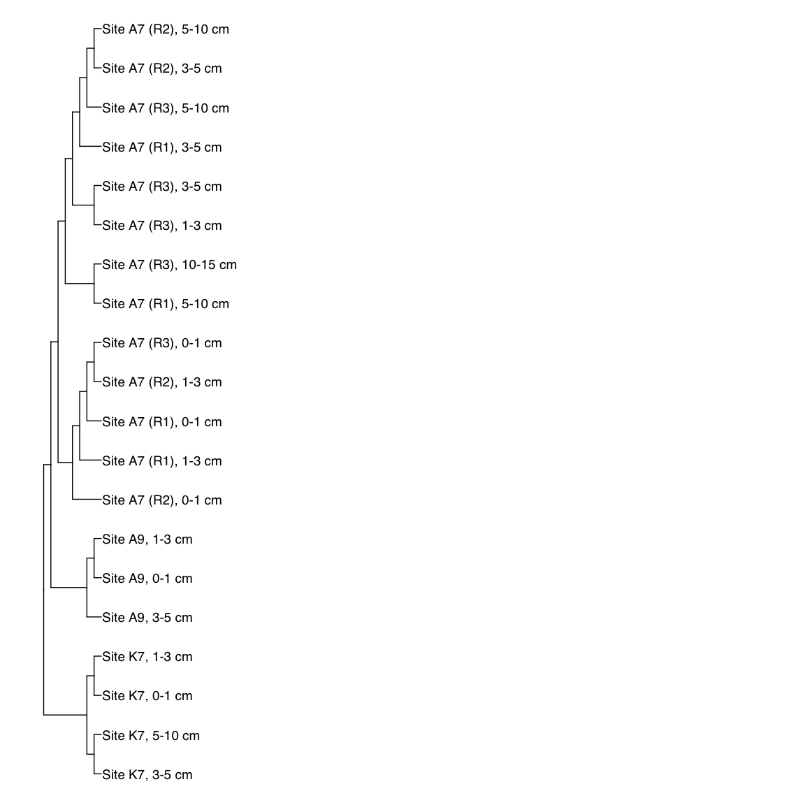
#dev.off()
# A7S_Bin_00119: gamma-2.2, SNV
A7S_Bin_00119_FST <- treeio::read.tree(here("NON_REDUNDANT_BINS/10_VAR_PROFILES/3_FST_SNV/FST_A7S_Bin_00119.newick"))
FST_simple <- full_join(A7S_Bin_00119_FST, meta[meta$Sample_ID %in% A7S_Bin_00119_FST$tip.label,],
by = c("label" = "Sample_ID"))
x_simple <- ggtree(FST_simple, branch.length="none") +
geom_tiplab(aes(label=Simple_labels), size=5, offset=0.1)
#svg(here::here("Export_figures/Fig_S5_A7S119_SNV_FST.svg"), width=10, height=12)
x_simple + xlim(0,100)
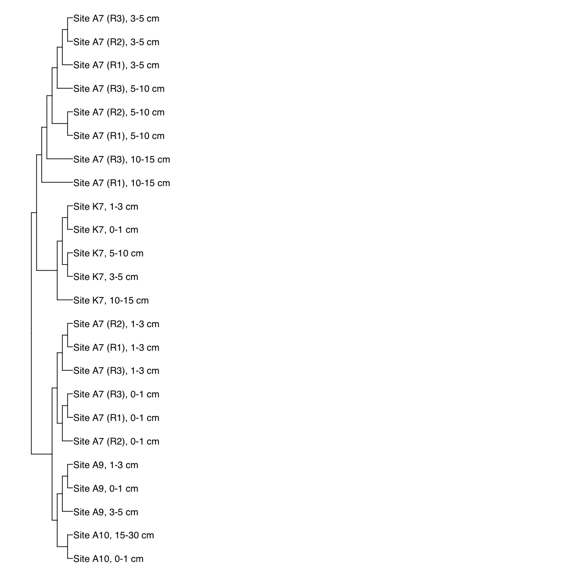
#dev.off()
Figure S6: FST-based trees for other theta
# A7D_Bin_00152: gamma-2.2, SNV
A7D_Bin_00152_FST <- treeio::read.tree(here("NON_REDUNDANT_BINS/10_VAR_PROFILES/3_FST_SNV/FST_A7D_Bin_00152.newick"))
FST_simple <- full_join(A7D_Bin_00152_FST, meta[meta$Sample_ID %in% A7D_Bin_00152_FST$tip.label,],
by = c("label" = "Sample_ID"))
x_simple <- ggtree(FST_simple, branch.length="none") +
geom_tiplab(aes(label=Simple_labels), size=5, offset=0.1)
#svg(here::here("Export_figures/Fig_S6_A7D152_SNV_FST.svg"), width=10, height=12)
x_simple + xlim(0,100)
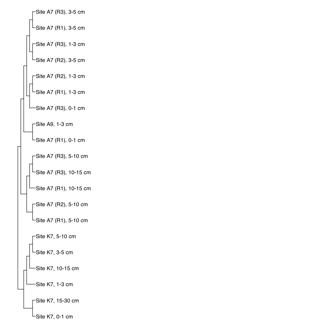
#dev.off()
# A7S_Bin_00118: gamma-2.2, SNV
A7S_Bin_00118_FST <- treeio::read.tree(here("NON_REDUNDANT_BINS/10_VAR_PROFILES/3_FST_SNV/FST_A7S_Bin_00118.newick"))
FST_simple <- full_join(A7S_Bin_00118_FST, meta[meta$Sample_ID %in% A7S_Bin_00118_FST$tip.label,],
by = c("label" = "Sample_ID"))
x_simple <- ggtree(FST_simple, branch.length="none") +
geom_tiplab(aes(label=Simple_labels), size=5, offset=0.1)
#svg(here::here("Export_figures/Fig_S6_A7S118_SNV_FST.svg"), width=10, height=12)
x_simple + xlim(0,100)
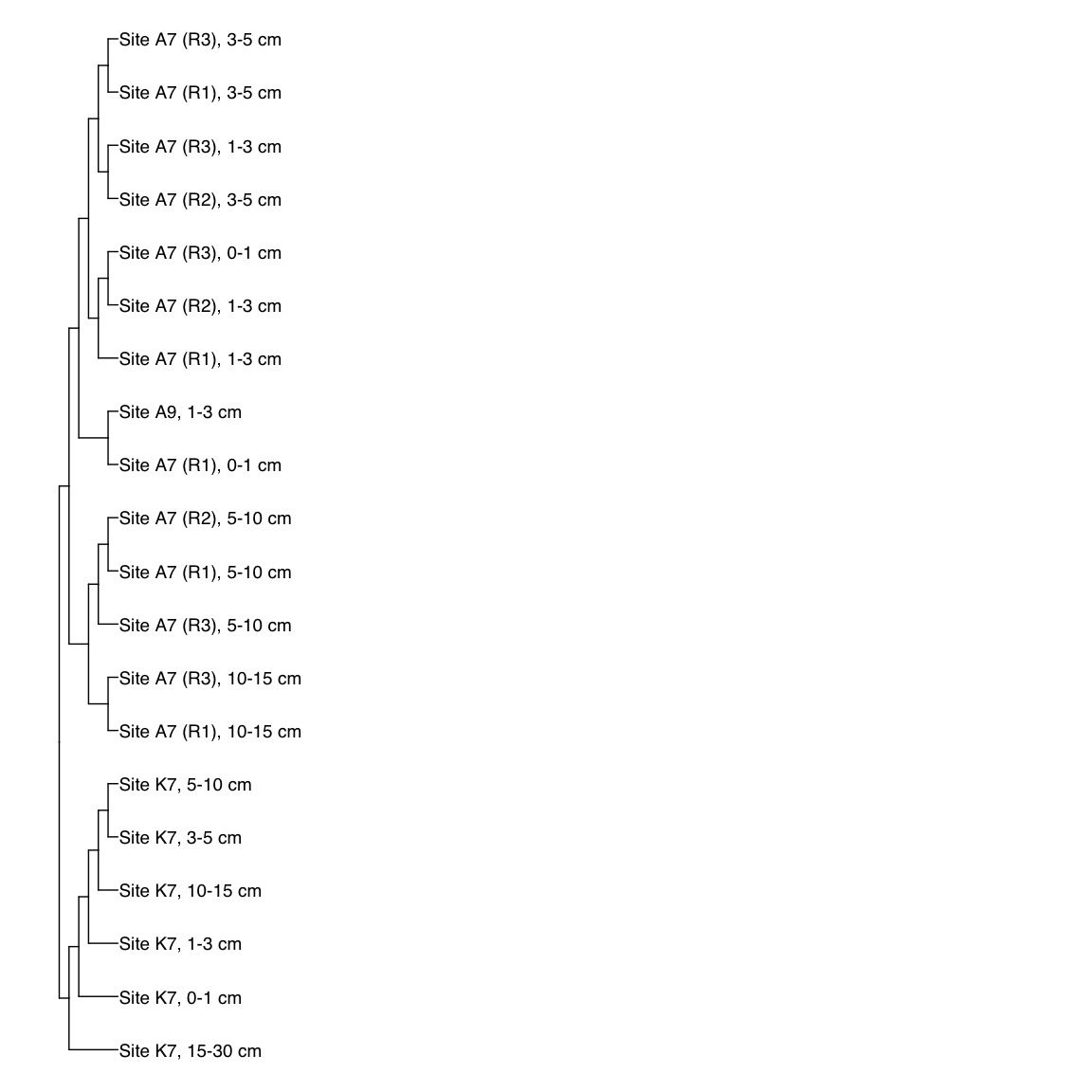
#dev.off()
# AK7_Bin_00081: gamma-2.2, SNV
AK7_Bin_00081_FST <- treeio::read.tree(here("NON_REDUNDANT_BINS/10_VAR_PROFILES/3_FST_SNV/FST_AK7_Bin_00081.newick"))
FST_simple <- full_join(AK7_Bin_00081_FST, meta[meta$Sample_ID %in% AK7_Bin_00081_FST$tip.label,],
by = c("label" = "Sample_ID"))
x_simple <- ggtree(FST_simple, branch.length="none") +
geom_tiplab(aes(label=Simple_labels), size=5, offset=0.1)
#svg(here::here("Export_figures/Fig_S6_AK781_SNV_FST.svg"), width=10, height=12)
x_simple + xlim(0,100)
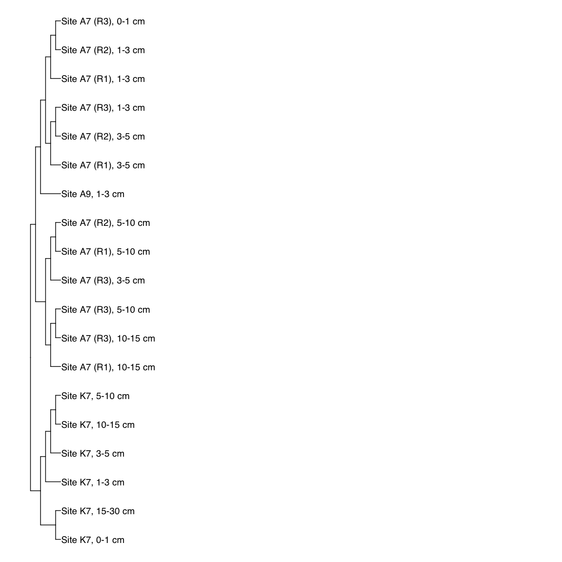
#dev.off()
# A7D_Bin_00162: gamma-2.2, SNV
A7D_Bin_00162_FST <- treeio::read.tree(here("NON_REDUNDANT_BINS/10_VAR_PROFILES/3_FST_SNV/FST_A7D_Bin_00162.newick"))
FST_simple <- full_join(A7D_Bin_00162_FST, meta[meta$Sample_ID %in% A7D_Bin_00162_FST$tip.label,],
by = c("label" = "Sample_ID"))
x_simple <- ggtree(FST_simple, branch.length="none") +
geom_tiplab(aes(label=Simple_labels), size=5, offset=0.1)
#svg(here::here("Export_figures/Fig_S6_A7D162_SNV_FST.svg"), width=10, height=12)
x_simple + xlim(0,100)
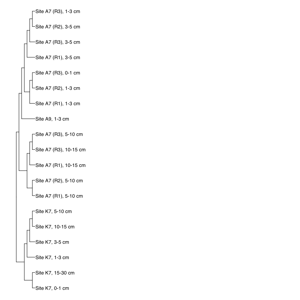
#dev.off()
Figure S7: Downcore evolution for other gamma-2.1
prepare_df_var <- function(MAG, clade){
df_var <- read.table(here::here(paste0("NON_REDUNDANT_BINS/10_VAR_PROFILES/2_SNV_files/SNVs_10dep_10cov_", MAG, ".txt", sep = "")),
sep = "\t", header = 1)
df_var <- left_join(df_var, meta, by = c("sample_id" = "Sample_ID"))
df_var <- df_var[df_var$Site == "A7", ]
# check that all samples have enough detection (aka they are part of the samples of interest)
print(unique(df_var$sample_id) %in% samples_of_interest[samples_of_interest$MAG_name == "AK7_Bin_00137",]$sample_id)
# filter to keep only variable positions
df_var <- df_var[df_var$departure_from_reference != 0 & df_var$departure_from_consensus != 0,]
# order
df_var$Horizon <- factor(df_var$Horizon, levels = flipped_horizon_order)
df_var$unique_pos_identifier <- as.character(df_var$unique_pos_identifier)
## Number of SNVs by kbp for each sample (NOT divided by coverage cf Matt Olm)
SNV_nb_df <- count_SNVs(df_var, MAG, clade)
SNV_nb_df$MAG <- MAG
return(list(df_var, SNV_nb_df))
}
clade_representative_list <- c("HKT_Bin_00027", "H3T_Bin_00167", "AK7_Bin_00137",
"H3D_Bin_00215", "HKT_Bin_00076", "HKT_Bin_00075")
# do it for each target MAG and join
SNV_nb_df_full <- data.frame(matrix(ncol=0,nrow=0))
df_shared_SNVs_long_full <- data.frame(matrix(ncol=0,nrow=0))
FST_A7_long_full <- data.frame(matrix(ncol=0,nrow=0))
df_cov_by_sample_A7_full <- data.frame(matrix(ncol=0,nrow=0))
for (i in (1:length(clade_representative_list))){
df_list <- downcore_plot(clade_representative_list[i], "amoA-NP-gamma-2.1")
FST_A7_long_full <- rbind(FST_A7_long_full, df_list[[1]])
df_cov_by_sample_A7_full <- rbind(df_cov_by_sample_A7_full, df_list[[2]])
df <- prepare_df_var(clade_representative_list[i], "amoA-NP-gamma-2.1")
df[[2]]$MAG <- clade_representative_list[i]
SNV_nb_df_full <- rbind(SNV_nb_df_full, df[[2]][, c(1:4,6:19)])
# % of shared SNVs between 2 samples and % of shared SNVs with same consensus nucleotide
df_shared_SNVs <- compute_shared_SNVs(df[[1]], "amoA-NP-gamma-2.1")
df_shared_SNVs$MAG_name <- clade_representative_list[i]
df_shared_SNVs_long_full <- rbind(df_shared_SNVs_long_full, df_shared_SNVs)
}
## [1] TRUE TRUE TRUE TRUE TRUE TRUE TRUE TRUE TRUE TRUE TRUE TRUE TRUE TRUE
## [1] TRUE TRUE TRUE TRUE TRUE TRUE TRUE TRUE TRUE TRUE TRUE TRUE TRUE TRUE
## [1] TRUE TRUE TRUE TRUE TRUE TRUE TRUE TRUE TRUE TRUE TRUE TRUE TRUE TRUE
## [1] TRUE TRUE TRUE TRUE TRUE TRUE TRUE TRUE TRUE TRUE TRUE TRUE TRUE TRUE
## [1] TRUE TRUE TRUE TRUE TRUE TRUE TRUE TRUE TRUE TRUE TRUE TRUE TRUE
## [1] TRUE TRUE TRUE TRUE TRUE TRUE TRUE TRUE TRUE TRUE TRUE TRUE TRUE TRUE
# order
FST_A7_long_full$Comparison_color <- paste0(FST_A7_long_full$Comparison, " ", FST_A7_long_full$Clade)
SNV_nb_df_full$Horizon <- factor(SNV_nb_df_full$Horizon, levels = flipped_horizon_order)
df_shared_SNVs_long_full$Sample1_horizon <- factor(df_shared_SNVs_long_full$Sample1_horizon, levels = flipped_horizon_order)
df_shared_SNVs_long_full$Sample2_horizon <- factor(df_shared_SNVs_long_full$Sample2_horizon, levels = flipped_horizon_order)
df_shared_SNVs_loooong <- pivot_longer(df_shared_SNVs_long_full, c(3,9))
# no 10-15 cm layer
FST_A7_long_full <- FST_A7_long_full[FST_A7_long_full$Sample1_horizon != "10_15" &
FST_A7_long_full$Sample2_horizon != "10_15", ]
df_cov_by_sample_A7_full <- df_cov_by_sample_A7_full[df_cov_by_sample_A7_full$Horizon != "10_15",]
df_shared_SNVs_loooong <- df_shared_SNVs_loooong[df_shared_SNVs_loooong$Sample1_horizon != "10_15" &
df_shared_SNVs_loooong$Sample2_horizon != "10_15",]
SNV_nb_df_full <- SNV_nb_df_full[SNV_nb_df_full$Horizon != "10_15",]
########### PLOT
# by horizon type
box <- ggplot(FST_A7_long_full, aes(x = Sample1_horizon, y = FST, fill = Comparison_color)) +
geom_boxplot(width = 0.5, linewidth = 0.5, position = position_dodge(0.7), alpha = 0.7) +
facet_grid(MAG_name~.) +
scale_x_discrete(breaks = flipped_horizon_order, labels = flipped_horizon_names) +
xlab("Sediment depth (cm)") + ylab("Fixation index") +
scale_fill_manual(values = scale_comparison) +
theme_bw() +
theme(axis.title.x = element_text(face = "bold", size = 14),
axis.title.y = element_text(face = "bold", size = 14),
axis.text.x = element_text(size = 12),
axis.text.y = element_text(size = 12),
axis.line.y = element_line(colour = "black"),
axis.line.x = element_line(colour = "black"),
strip.text = element_blank()) +
coord_flip()
bubble <- ggplot(df_cov_by_sample_A7_full, aes(x = Horizon, y = factor(Site))) +
geom_point(aes(size = mean_coverage, fill = Clade), alpha = 0.3, shape = 21) +
facet_grid(MAG_name~.) +
geom_text(aes(label = label)) +
scale_size(range = c(1, 20), name="Mean coverage") +
ylab("Mean coverage") + scale_fill_manual(values = scale_amoA, guide = guide_legend(override.aes = list(size = 8))) +
theme_bw() +
theme(axis.title.x = element_text(face = "bold", size = 14),
axis.title.y = element_blank(),
axis.text = element_blank(),
panel.grid = element_blank(),
panel.border = element_blank(),
axis.line = element_blank(),
axis.ticks = element_blank(),
strip.text = element_blank()) +
coord_flip()
### with bubble
comp_plot <- ggplot(df_shared_SNVs_loooong, aes(x = Sample1_horizon, y = value, fill = Clade, pattern = name)) +
geom_boxplot_pattern(width = 1, linewidth = 0.5, pattern_angle = 45,
pattern_fill = "white", pattern_color = "white", alpha = 0.7) +
facet_grid(MAG_name~.) +
xlab("Sediment depth (cm)") + ylab("SNV positions (%)") +
scale_x_discrete(breaks = flipped_horizon_order, labels = flipped_horizon_names) +
scale_fill_manual(values = scale_amoA) +
scale_pattern_manual(values = c(Percent_pos_shared = "stripe", Shared_same_consensus = "none")) +
theme_bw() +
theme(axis.title.x = element_text(face = "bold", size = 14),
axis.text = element_text(size = 12),
axis.title.y = element_blank(),
strip.text = element_blank()) +
guides(pattern = guide_legend(override.aes = list(fill = "black", pattern_fill = "white", pattern_color = "white")),
fill = guide_legend(override.aes = list(pattern = "none"))) +
coord_flip()
SNV_nb_df_full$Y <- "all"
SNV_nb_df_full$SNV_label <- paste0(SNV_nb_df_full$mean, " ± ", SNV_nb_df_full$sd)
nb_bubble <- ggplot(SNV_nb_df_full, aes(x = Horizon, y = factor(Y))) +
geom_point(aes(size = mean, fill = Clade), alpha = 0.3, shape = 21) +
facet_grid(MAG~.) +
scale_size(range = c(1, 20), name="SNV number / kbp") +
geom_text(aes(label = SNV_label)) + ylab("SNV density") +
scale_fill_manual(values = scale_amoA, guide = guide_legend(override.aes = list(size = 8))) +
theme_bw() +
theme(axis.title.x = element_text(face = "bold", size = 14),
axis.title.y = element_blank(),
axis.text = element_blank(),
axis.ticks = element_blank(),
legend.title = element_text(size = 14, face = "bold"),
legend.text = element_text(size = 12),
panel.grid = element_blank(),
panel.border = element_blank(),
strip.text.x = element_text(size = 14)) +
coord_flip()
### Full plot
#svg(here::here("Export_figures/Fig_S7_with_legend.svg"), width=18, height=12)
box + bubble + comp_plot + nb_bubble + plot_layout(width = c(2,1,2,1), guides = 'collect')
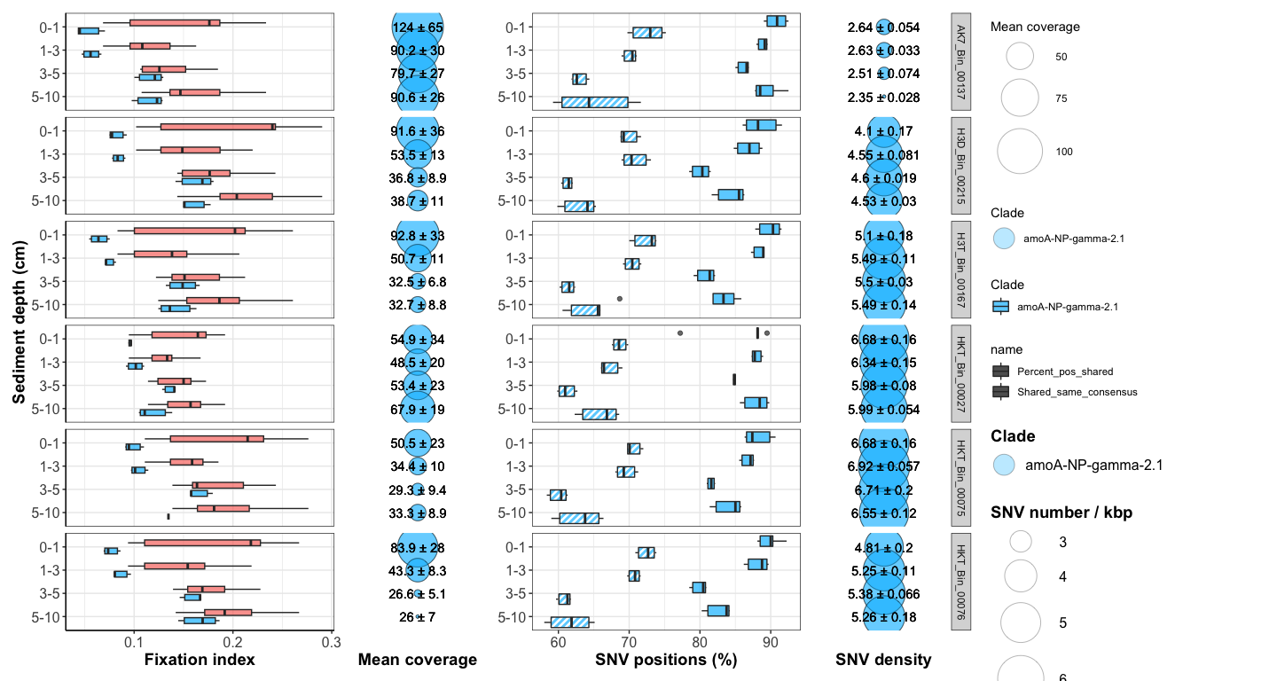
#dev.off()
# correlation of FST distance with shared SNVs ?
correlation <- right_join(FST_A7_long_full, df_shared_SNVs_long_full, by = c("Sample_1" = "Sample_ID_1", "Sample_2" = "Sample_ID_2", "Sample1_horizon", "Sample2_horizon", "Sample1_core", "Sample2_core", "Clade", "MAG_name"))
by(correlation, correlation$MAG_name, function(x) summary(lm(x$FST ~ x$Percent_pos_shared)))
## correlation$MAG_name: AK7_Bin_00137
##
## Call:
## lm(formula = x$FST ~ x$Percent_pos_shared)
##
## Residuals:
## Min 1Q Median 3Q Max
## -0.022346 -0.011907 -0.006135 0.010627 0.035346
##
## Coefficients:
## Estimate Std. Error t value Pr(>|t|)
## (Intercept) 0.4892148 0.0501898 9.747 1.92e-09 ***
## x$Percent_pos_shared -0.0059601 0.0007395 -8.060 5.22e-08 ***
## ---
## Signif. codes: 0 '***' 0.001 '**' 0.01 '*' 0.05 '.' 0.1 ' ' 1
##
## Residual standard error: 0.01744 on 22 degrees of freedom
## (2 observations deleted due to missingness)
## Multiple R-squared: 0.747, Adjusted R-squared: 0.7355
## F-statistic: 64.96 on 1 and 22 DF, p-value: 5.218e-08
##
## ------------------------------------------------------------
## correlation$MAG_name: H3D_Bin_00215
##
## Call:
## lm(formula = x$FST ~ x$Percent_pos_shared)
##
## Residuals:
## Min 1Q Median 3Q Max
## -0.018527 -0.009597 0.002586 0.007116 0.019338
##
## Coefficients:
## Estimate Std. Error t value Pr(>|t|)
## (Intercept) 0.7071065 0.0384842 18.37 7.78e-15 ***
## x$Percent_pos_shared -0.0088260 0.0005795 -15.23 3.61e-13 ***
## ---
## Signif. codes: 0 '***' 0.001 '**' 0.01 '*' 0.05 '.' 0.1 ' ' 1
##
## Residual standard error: 0.0126 on 22 degrees of freedom
## (2 observations deleted due to missingness)
## Multiple R-squared: 0.9134, Adjusted R-squared: 0.9094
## F-statistic: 232 on 1 and 22 DF, p-value: 3.611e-13
##
## ------------------------------------------------------------
## correlation$MAG_name: H3T_Bin_00167
##
## Call:
## lm(formula = x$FST ~ x$Percent_pos_shared)
##
## Residuals:
## Min 1Q Median 3Q Max
## -0.013360 -0.008162 0.002210 0.003953 0.016959
##
## Coefficients:
## Estimate Std. Error t value Pr(>|t|)
## (Intercept) 0.6525340 0.0248774 26.23 <2e-16 ***
## x$Percent_pos_shared -0.0081300 0.0003701 -21.97 <2e-16 ***
## ---
## Signif. codes: 0 '***' 0.001 '**' 0.01 '*' 0.05 '.' 0.1 ' ' 1
##
## Residual standard error: 0.008683 on 22 degrees of freedom
## (2 observations deleted due to missingness)
## Multiple R-squared: 0.9564, Adjusted R-squared: 0.9544
## F-statistic: 482.5 on 1 and 22 DF, p-value: < 2.2e-16
##
## ------------------------------------------------------------
## correlation$MAG_name: HKT_Bin_00027
##
## Call:
## lm(formula = x$FST ~ x$Percent_pos_shared)
##
## Residuals:
## Min 1Q Median 3Q Max
## -0.007474 -0.003525 -0.001028 0.003593 0.007298
##
## Coefficients:
## Estimate Std. Error t value Pr(>|t|)
## (Intercept) 0.4672821 0.0198964 23.49 < 2e-16 ***
## x$Percent_pos_shared -0.0053904 0.0003023 -17.83 1.45e-14 ***
## ---
## Signif. codes: 0 '***' 0.001 '**' 0.01 '*' 0.05 '.' 0.1 ' ' 1
##
## Residual standard error: 0.004838 on 22 degrees of freedom
## (2 observations deleted due to missingness)
## Multiple R-squared: 0.9353, Adjusted R-squared: 0.9323
## F-statistic: 317.9 on 1 and 22 DF, p-value: 1.45e-14
##
## ------------------------------------------------------------
## correlation$MAG_name: HKT_Bin_00075
##
## Call:
## lm(formula = x$FST ~ x$Percent_pos_shared)
##
## Residuals:
## Min 1Q Median 3Q Max
## -0.0112752 -0.0056708 0.0009676 0.0045888 0.0090684
##
## Coefficients:
## Estimate Std. Error t value Pr(>|t|)
## (Intercept) 0.5445987 0.0200362 27.18 4.57e-16 ***
## x$Percent_pos_shared -0.0063118 0.0002998 -21.06 3.96e-14 ***
## ---
## Signif. codes: 0 '***' 0.001 '**' 0.01 '*' 0.05 '.' 0.1 ' ' 1
##
## Residual standard error: 0.006233 on 18 degrees of freedom
## (6 observations deleted due to missingness)
## Multiple R-squared: 0.961, Adjusted R-squared: 0.9588
## F-statistic: 443.3 on 1 and 18 DF, p-value: 3.957e-14
##
## ------------------------------------------------------------
## correlation$MAG_name: HKT_Bin_00076
##
## Call:
## lm(formula = x$FST ~ x$Percent_pos_shared)
##
## Residuals:
## Min 1Q Median 3Q Max
## -0.012361 -0.005489 -0.001337 0.005679 0.012200
##
## Coefficients:
## Estimate Std. Error t value Pr(>|t|)
## (Intercept) 0.635341 0.019664 32.31 <2e-16 ***
## x$Percent_pos_shared -0.007723 0.000295 -26.18 <2e-16 ***
## ---
## Signif. codes: 0 '***' 0.001 '**' 0.01 '*' 0.05 '.' 0.1 ' ' 1
##
## Residual standard error: 0.007898 on 22 degrees of freedom
## Multiple R-squared: 0.9689, Adjusted R-squared: 0.9675
## F-statistic: 685.4 on 1 and 22 DF, p-value: < 2.2e-16
by(correlation, correlation$MAG_name, function(x) summary(lm(x$FST ~ x$Shared_same_consensus)))
## correlation$MAG_name: AK7_Bin_00137
##
## Call:
## lm(formula = x$FST ~ x$Shared_same_consensus)
##
## Residuals:
## Min 1Q Median 3Q Max
## -0.031640 -0.023393 -0.009112 0.025052 0.047436
##
## Coefficients:
## Estimate Std. Error t value Pr(>|t|)
## (Intercept) 0.93911 0.23804 3.945 0.000689 ***
## x$Shared_same_consensus -0.00961 0.00268 -3.586 0.001646 **
## ---
## Signif. codes: 0 '***' 0.001 '**' 0.01 '*' 0.05 '.' 0.1 ' ' 1
##
## Residual standard error: 0.02754 on 22 degrees of freedom
## (2 observations deleted due to missingness)
## Multiple R-squared: 0.3689, Adjusted R-squared: 0.3402
## F-statistic: 12.86 on 1 and 22 DF, p-value: 0.001646
##
## ------------------------------------------------------------
## correlation$MAG_name: H3D_Bin_00215
##
## Call:
## lm(formula = x$FST ~ x$Shared_same_consensus)
##
## Residuals:
## Min 1Q Median 3Q Max
## -0.033315 -0.018304 -0.003017 0.018129 0.039461
##
## Coefficients:
## Estimate Std. Error t value Pr(>|t|)
## (Intercept) 0.908527 0.112165 8.100 4.80e-08 ***
## x$Shared_same_consensus -0.009248 0.001318 -7.016 4.85e-07 ***
## ---
## Signif. codes: 0 '***' 0.001 '**' 0.01 '*' 0.05 '.' 0.1 ' ' 1
##
## Residual standard error: 0.02379 on 22 degrees of freedom
## (2 observations deleted due to missingness)
## Multiple R-squared: 0.6911, Adjusted R-squared: 0.6771
## F-statistic: 49.23 on 1 and 22 DF, p-value: 4.848e-07
##
## ------------------------------------------------------------
## correlation$MAG_name: H3T_Bin_00167
##
## Call:
## lm(formula = x$FST ~ x$Shared_same_consensus)
##
## Residuals:
## Min 1Q Median 3Q Max
## -0.08180 -0.01325 -0.01230 0.02177 0.03604
##
## Coefficients:
## Estimate Std. Error t value Pr(>|t|)
## (Intercept) 0.618908 0.089456 6.919 6.02e-07 ***
## x$Shared_same_consensus -0.006009 0.001049 -5.728 9.23e-06 ***
## ---
## Signif. codes: 0 '***' 0.001 '**' 0.01 '*' 0.05 '.' 0.1 ' ' 1
##
## Residual standard error: 0.02635 on 22 degrees of freedom
## (2 observations deleted due to missingness)
## Multiple R-squared: 0.5986, Adjusted R-squared: 0.5803
## F-statistic: 32.81 on 1 and 22 DF, p-value: 9.233e-06
##
## ------------------------------------------------------------
## correlation$MAG_name: HKT_Bin_00027
##
## Call:
## lm(formula = x$FST ~ x$Shared_same_consensus)
##
## Residuals:
## Min 1Q Median 3Q Max
## -0.045790 -0.011952 -0.000705 0.013202 0.022526
##
## Coefficients:
## Estimate Std. Error t value Pr(>|t|)
## (Intercept) 0.356629 0.117150 3.044 0.00595 **
## x$Shared_same_consensus -0.002806 0.001348 -2.081 0.04932 *
## ---
## Signif. codes: 0 '***' 0.001 '**' 0.01 '*' 0.05 '.' 0.1 ' ' 1
##
## Residual standard error: 0.01738 on 22 degrees of freedom
## (2 observations deleted due to missingness)
## Multiple R-squared: 0.1644, Adjusted R-squared: 0.1264
## F-statistic: 4.329 on 1 and 22 DF, p-value: 0.04932
##
## ------------------------------------------------------------
## correlation$MAG_name: HKT_Bin_00075
##
## Call:
## lm(formula = x$FST ~ x$Shared_same_consensus)
##
## Residuals:
## Min 1Q Median 3Q Max
## -0.011371 -0.009205 -0.003079 0.011882 0.016996
##
## Coefficients:
## Estimate Std. Error t value Pr(>|t|)
## (Intercept) 0.9478597 0.0696763 13.60 6.53e-11 ***
## x$Shared_same_consensus -0.0096354 0.0008142 -11.84 6.31e-10 ***
## ---
## Signif. codes: 0 '***' 0.001 '**' 0.01 '*' 0.05 '.' 0.1 ' ' 1
##
## Residual standard error: 0.01065 on 18 degrees of freedom
## (6 observations deleted due to missingness)
## Multiple R-squared: 0.8861, Adjusted R-squared: 0.8798
## F-statistic: 140.1 on 1 and 18 DF, p-value: 6.308e-10
##
## ------------------------------------------------------------
## correlation$MAG_name: HKT_Bin_00076
##
## Call:
## lm(formula = x$FST ~ x$Shared_same_consensus)
##
## Residuals:
## Min 1Q Median 3Q Max
## -0.020204 -0.012124 -0.000697 0.009143 0.038039
##
## Coefficients:
## Estimate Std. Error t value Pr(>|t|)
## (Intercept) 0.9178912 0.0690182 13.30 5.39e-12 ***
## x$Shared_same_consensus -0.0093411 0.0008093 -11.54 8.36e-11 ***
## ---
## Signif. codes: 0 '***' 0.001 '**' 0.01 '*' 0.05 '.' 0.1 ' ' 1
##
## Residual standard error: 0.01686 on 22 degrees of freedom
## Multiple R-squared: 0.8583, Adjusted R-squared: 0.8518
## F-statistic: 133.2 on 1 and 22 DF, p-value: 8.36e-11
There is no supplementary figure for gamma-2.2 because HKT_Bin_00022 does not appear in site A7 when taking into account detection
Figure S8: Downcore evolution for other delta
clade_representative_list <- c("A7D_Bin_00065", "A9S_Bin_00058", "A7D_Bin_00052", "AK7_Bin_00037", "AK7_Bin_00136", "A7S_Bin_00119")
# do it for each target MAG and join
SNV_nb_df_full <- data.frame(matrix(ncol=0,nrow=0))
df_shared_SNVs_long_full <- data.frame(matrix(ncol=0,nrow=0))
FST_A7_long_full <- data.frame(matrix(ncol=0,nrow=0))
df_cov_by_sample_A7_full <- data.frame(matrix(ncol=0,nrow=0))
for (i in (1:length(clade_representative_list))){
df_list <- downcore_plot(clade_representative_list[i], "amoA-NP-delta")
FST_A7_long_full <- rbind(FST_A7_long_full, df_list[[1]])
df_cov_by_sample_A7_full <- rbind(df_cov_by_sample_A7_full, df_list[[2]])
df <- prepare_df_var(clade_representative_list[i], "amoA-NP-delta")
df[[2]]$MAG <- clade_representative_list[i]
SNV_nb_df_full <- rbind(SNV_nb_df_full, df[[2]][, c(1:4,6:19)])
# % of shared SNVs between 2 samples and % of shared SNVs with same consensus nucleotide
df_shared_SNVs <- compute_shared_SNVs(df[[1]], "amoA-NP-delta")
df_shared_SNVs$MAG_name <- clade_representative_list[i]
df_shared_SNVs_long_full <- rbind(df_shared_SNVs_long_full, df_shared_SNVs)
}
## [1] TRUE TRUE TRUE TRUE TRUE TRUE TRUE TRUE TRUE TRUE TRUE TRUE TRUE TRUE
## [1] TRUE TRUE TRUE TRUE TRUE TRUE TRUE TRUE TRUE TRUE TRUE TRUE
## [1] TRUE TRUE TRUE TRUE TRUE TRUE TRUE TRUE TRUE TRUE TRUE TRUE TRUE TRUE
## [1] TRUE TRUE TRUE TRUE TRUE TRUE TRUE TRUE TRUE TRUE TRUE TRUE TRUE TRUE
## [1] TRUE TRUE TRUE TRUE TRUE TRUE TRUE TRUE TRUE TRUE TRUE TRUE TRUE TRUE
## [1] TRUE TRUE TRUE TRUE TRUE TRUE TRUE TRUE TRUE TRUE TRUE TRUE TRUE TRUE
# order
FST_A7_long_full$Comparison_color <- paste0(FST_A7_long_full$Comparison, " ", FST_A7_long_full$Clade)
SNV_nb_df_full$Horizon <- factor(SNV_nb_df_full$Horizon, levels = flipped_horizon_order)
df_shared_SNVs_long_full$Sample1_horizon <- factor(df_shared_SNVs_long_full$Sample1_horizon, levels = flipped_horizon_order)
df_shared_SNVs_long_full$Sample2_horizon <- factor(df_shared_SNVs_long_full$Sample2_horizon, levels = flipped_horizon_order)
df_shared_SNVs_loooong <- pivot_longer(df_shared_SNVs_long_full, c(3,9))
# no 10-15 cm layer
FST_A7_long_full <- FST_A7_long_full[FST_A7_long_full$Sample1_horizon != "10_15" &
FST_A7_long_full$Sample2_horizon != "10_15", ]
df_cov_by_sample_A7_full <- df_cov_by_sample_A7_full[df_cov_by_sample_A7_full$Horizon != "10_15",]
df_shared_SNVs_loooong <- df_shared_SNVs_loooong[df_shared_SNVs_loooong$Sample1_horizon != "10_15" &
df_shared_SNVs_loooong$Sample2_horizon != "10_15",]
SNV_nb_df_full <- SNV_nb_df_full[SNV_nb_df_full$Horizon != "10_15",]
#################### PLOT
# by horizon type
box <- ggplot(FST_A7_long_full, aes(x = Sample1_horizon, y = FST, fill = Comparison_color)) +
geom_boxplot(width = 0.5, linewidth = 0.5, position = position_dodge(0.7), alpha = 0.7) +
facet_grid(MAG_name~.) +
scale_x_discrete(breaks = flipped_horizon_order, labels = flipped_horizon_names) +
xlab("Sediment depth (cm)") + ylab("Fixation index") +
scale_fill_manual(values = scale_comparison) +
theme_bw() +
theme(axis.title.x = element_text(face = "bold", size = 14),
axis.title.y = element_text(face = "bold", size = 14),
axis.text.x = element_text(size = 12),
axis.text.y = element_text(size = 12),
axis.line.y = element_line(colour = "black"),
axis.line.x = element_line(colour = "black"),
strip.text = element_blank()) +
coord_flip()
bubble <- ggplot(df_cov_by_sample_A7_full, aes(x = Horizon, y = factor(Site))) +
geom_point(aes(size = mean_coverage, fill = Clade), alpha = 0.3, shape = 21) +
facet_grid(MAG_name~.) +
geom_text(aes(label = label)) +
scale_size(range = c(1, 20), name="Mean coverage") +
ylab("Mean coverage") + scale_fill_manual(values = scale_amoA, guide = guide_legend(override.aes = list(size = 8))) +
theme_bw() +
theme(axis.title.x = element_text(face = "bold", size = 14),
axis.title.y = element_blank(),
axis.text = element_blank(),
panel.grid = element_blank(),
panel.border = element_blank(),
axis.line = element_blank(),
axis.ticks = element_blank(),
strip.text = element_blank()) +
coord_flip()
### with bubble
comp_plot <- ggplot(df_shared_SNVs_loooong, aes(x = Sample1_horizon, y = value, fill = Clade, pattern = name)) +
geom_boxplot_pattern(width = 1, linewidth = 0.5, pattern_angle = 45,
pattern_fill = "white", pattern_color = "white", alpha = 0.7) +
facet_grid(MAG_name~.) +
xlab("Sediment depth (cm)") + ylab("SNV positions (%)") +
scale_x_discrete(breaks = flipped_horizon_order, labels = flipped_horizon_names) +
scale_fill_manual(values = scale_amoA) +
scale_pattern_manual(values = c(Percent_pos_shared = "stripe", Shared_same_consensus = "none")) +
theme_bw() +
theme(axis.title.x = element_text(face = "bold", size = 14),
axis.text = element_text(size = 12),
axis.title.y = element_blank(),
strip.text = element_blank()) +
guides(pattern = guide_legend(override.aes = list(fill = "black", pattern_fill = "white", pattern_color = "white")),
fill = guide_legend(override.aes = list(pattern = "none"))) +
coord_flip()
SNV_nb_df_full$Y <- "all"
SNV_nb_df_full$SNV_label <- paste0(SNV_nb_df_full$mean, " ± ", SNV_nb_df_full$sd)
nb_bubble <- ggplot(SNV_nb_df_full, aes(x = Horizon, y = factor(Y))) +
geom_point(aes(size = mean, fill = Clade), alpha = 0.3, shape = 21) +
facet_grid(MAG~.) +
scale_size(range = c(1, 20), name="SNV number / kbp") +
geom_text(aes(label = SNV_label)) + ylab("SNV density") +
scale_fill_manual(values = scale_amoA, guide = guide_legend(override.aes = list(size = 8))) +
theme_bw() +
theme(axis.title.x = element_text(face = "bold", size = 14),
axis.title.y = element_blank(),
axis.text = element_blank(),
axis.ticks = element_blank(),
legend.title = element_text(size = 14, face = "bold"),
legend.text = element_text(size = 12),
panel.grid = element_blank(),
panel.border = element_blank(),
strip.text.x = element_text(size = 14)) +
coord_flip()
### Full plot
#svg(here::here("Export_figures/Fig_S8_with_legend.svg"), width=18, height=12)
box + bubble + comp_plot + nb_bubble + plot_layout(width = c(2,1,2,1), guides = 'collect')
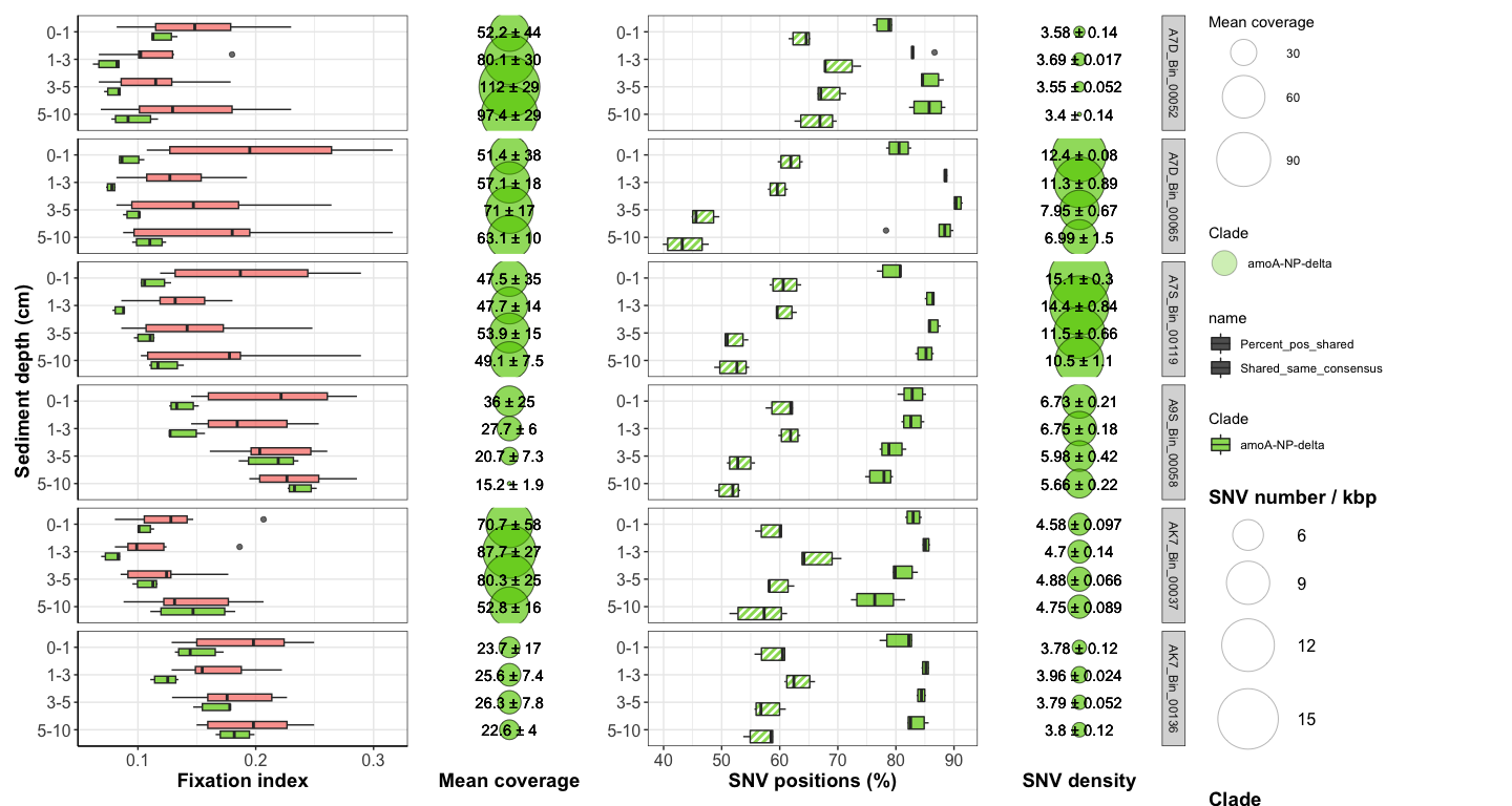
#dev.off()
# correlation of FST distance with shared SNVs ?
correlation <- right_join(FST_A7_long_full, df_shared_SNVs_long_full, by = c("Sample_1" = "Sample_ID_1", "Sample_2" = "Sample_ID_2", "Sample1_horizon", "Sample2_horizon", "Sample1_core", "Sample2_core", "Clade", "MAG_name"))
by(correlation, correlation$MAG_name, function(x) summary(lm(x$FST ~ x$Percent_pos_shared)))
## correlation$MAG_name: A7D_Bin_00052
##
## Call:
## lm(formula = x$FST ~ x$Percent_pos_shared)
##
## Residuals:
## Min 1Q Median 3Q Max
## -0.0112626 -0.0048319 -0.0007878 0.0056620 0.0094488
##
## Coefficients:
## Estimate Std. Error t value Pr(>|t|)
## (Intercept) 0.4746872 0.0286531 16.57 6.55e-14 ***
## x$Percent_pos_shared -0.0056921 0.0004265 -13.35 5.02e-12 ***
## ---
## Signif. codes: 0 '***' 0.001 '**' 0.01 '*' 0.05 '.' 0.1 ' ' 1
##
## Residual standard error: 0.007072 on 22 degrees of freedom
## (2 observations deleted due to missingness)
## Multiple R-squared: 0.8901, Adjusted R-squared: 0.8851
## F-statistic: 178.1 on 1 and 22 DF, p-value: 5.024e-12
##
## ------------------------------------------------------------
## correlation$MAG_name: A7D_Bin_00065
##
## Call:
## lm(formula = x$FST ~ x$Percent_pos_shared)
##
## Residuals:
## Min 1Q Median 3Q Max
## -0.012022 -0.005810 -0.003079 0.004625 0.020618
##
## Coefficients:
## Estimate Std. Error t value Pr(>|t|)
## (Intercept) 0.1648446 0.0127767 12.902 9.76e-12 ***
## x$Percent_pos_shared -0.0013411 0.0002385 -5.624 1.18e-05 ***
## ---
## Signif. codes: 0 '***' 0.001 '**' 0.01 '*' 0.05 '.' 0.1 ' ' 1
##
## Residual standard error: 0.009601 on 22 degrees of freedom
## (2 observations deleted due to missingness)
## Multiple R-squared: 0.5897, Adjusted R-squared: 0.5711
## F-statistic: 31.62 on 1 and 22 DF, p-value: 1.181e-05
##
## ------------------------------------------------------------
## correlation$MAG_name: A7S_Bin_00119
##
## Call:
## lm(formula = x$FST ~ x$Percent_pos_shared)
##
## Residuals:
## Min 1Q Median 3Q Max
## -0.013954 -0.011057 -0.002623 0.009647 0.025959
##
## Coefficients:
## Estimate Std. Error t value Pr(>|t|)
## (Intercept) 0.2340690 0.0311608 7.512 1.65e-07 ***
## x$Percent_pos_shared -0.0022638 0.0005506 -4.111 0.00046 ***
## ---
## Signif. codes: 0 '***' 0.001 '**' 0.01 '*' 0.05 '.' 0.1 ' ' 1
##
## Residual standard error: 0.01304 on 22 degrees of freedom
## (2 observations deleted due to missingness)
## Multiple R-squared: 0.4345, Adjusted R-squared: 0.4088
## F-statistic: 16.9 on 1 and 22 DF, p-value: 0.0004599
##
## ------------------------------------------------------------
## correlation$MAG_name: A9S_Bin_00058
##
## Call:
## lm(formula = x$FST ~ x$Percent_pos_shared)
##
## Residuals:
## Min 1Q Median 3Q Max
## -0.0212933 -0.0044078 0.0005015 0.0052280 0.0126916
##
## Coefficients:
## Estimate Std. Error t value Pr(>|t|)
## (Intercept) 0.7180320 0.0210552 34.10 <2e-16 ***
## x$Percent_pos_shared -0.0094696 0.0003701 -25.59 <2e-16 ***
## ---
## Signif. codes: 0 '***' 0.001 '**' 0.01 '*' 0.05 '.' 0.1 ' ' 1
##
## Residual standard error: 0.008909 on 22 degrees of freedom
## Multiple R-squared: 0.9675, Adjusted R-squared: 0.966
## F-statistic: 654.8 on 1 and 22 DF, p-value: < 2.2e-16
##
## ------------------------------------------------------------
## correlation$MAG_name: AK7_Bin_00037
##
## Call:
## lm(formula = x$FST ~ x$Percent_pos_shared)
##
## Residuals:
## Min 1Q Median 3Q Max
## -0.021211 -0.009160 -0.004798 0.008972 0.022922
##
## Coefficients:
## Estimate Std. Error t value Pr(>|t|)
## (Intercept) 0.4463828 0.0364669 12.241 2.71e-11 ***
## x$Percent_pos_shared -0.0055856 0.0006032 -9.261 4.79e-09 ***
## ---
## Signif. codes: 0 '***' 0.001 '**' 0.01 '*' 0.05 '.' 0.1 ' ' 1
##
## Residual standard error: 0.01372 on 22 degrees of freedom
## (2 observations deleted due to missingness)
## Multiple R-squared: 0.7958, Adjusted R-squared: 0.7866
## F-statistic: 85.76 on 1 and 22 DF, p-value: 4.792e-09
##
## ------------------------------------------------------------
## correlation$MAG_name: AK7_Bin_00136
##
## Call:
## lm(formula = x$FST ~ x$Percent_pos_shared)
##
## Residuals:
## Min 1Q Median 3Q Max
## -0.0115565 -0.0074901 -0.0000557 0.0048947 0.0205036
##
## Coefficients:
## Estimate Std. Error t value Pr(>|t|)
## (Intercept) 0.5966537 0.0340436 17.53 2.06e-14 ***
## x$Percent_pos_shared -0.0074430 0.0005737 -12.97 8.77e-12 ***
## ---
## Signif. codes: 0 '***' 0.001 '**' 0.01 '*' 0.05 '.' 0.1 ' ' 1
##
## Residual standard error: 0.009263 on 22 degrees of freedom
## (2 observations deleted due to missingness)
## Multiple R-squared: 0.8844, Adjusted R-squared: 0.8791
## F-statistic: 168.3 on 1 and 22 DF, p-value: 8.77e-12
by(correlation, correlation$MAG_name, function(x) summary(lm(x$FST ~ x$Shared_same_consensus)))
## correlation$MAG_name: A7D_Bin_00052
##
## Call:
## lm(formula = x$FST ~ x$Shared_same_consensus)
##
## Residuals:
## Min 1Q Median 3Q Max
## -0.033148 -0.005704 -0.001306 0.004558 0.022440
##
## Coefficients:
## Estimate Std. Error t value Pr(>|t|)
## (Intercept) 0.461266 0.062624 7.366 2.26e-07 ***
## x$Shared_same_consensus -0.004429 0.000752 -5.890 6.30e-06 ***
## ---
## Signif. codes: 0 '***' 0.001 '**' 0.01 '*' 0.05 '.' 0.1 ' ' 1
##
## Residual standard error: 0.01329 on 22 degrees of freedom
## (2 observations deleted due to missingness)
## Multiple R-squared: 0.6119, Adjusted R-squared: 0.5943
## F-statistic: 34.69 on 1 and 22 DF, p-value: 6.301e-06
##
## ------------------------------------------------------------
## correlation$MAG_name: A7D_Bin_00065
##
## Call:
## lm(formula = x$FST ~ x$Shared_same_consensus)
##
## Residuals:
## Min 1Q Median 3Q Max
## -0.020823 -0.011011 -0.002787 0.008425 0.030169
##
## Coefficients:
## Estimate Std. Error t value Pr(>|t|)
## (Intercept) 9.910e-02 6.056e-02 1.636 0.116
## x$Shared_same_consensus -6.069e-05 6.980e-04 -0.087 0.931
##
## Residual standard error: 0.01499 on 22 degrees of freedom
## (2 observations deleted due to missingness)
## Multiple R-squared: 0.0003435, Adjusted R-squared: -0.0451
## F-statistic: 0.00756 on 1 and 22 DF, p-value: 0.9315
##
## ------------------------------------------------------------
## correlation$MAG_name: A7S_Bin_00119
##
## Call:
## lm(formula = x$FST ~ x$Shared_same_consensus)
##
## Residuals:
## Min 1Q Median 3Q Max
## -0.0224488 -0.0121416 0.0008533 0.0095800 0.0303259
##
## Coefficients:
## Estimate Std. Error t value Pr(>|t|)
## (Intercept) 0.322449 0.084894 3.798 0.000985 ***
## x$Shared_same_consensus -0.002566 0.001008 -2.546 0.018402 *
## ---
## Signif. codes: 0 '***' 0.001 '**' 0.01 '*' 0.05 '.' 0.1 ' ' 1
##
## Residual standard error: 0.01524 on 22 degrees of freedom
## (2 observations deleted due to missingness)
## Multiple R-squared: 0.2276, Adjusted R-squared: 0.1925
## F-statistic: 6.484 on 1 and 22 DF, p-value: 0.0184
##
## ------------------------------------------------------------
## correlation$MAG_name: A9S_Bin_00058
##
## Call:
## lm(formula = x$FST ~ x$Shared_same_consensus)
##
## Residuals:
## Min 1Q Median 3Q Max
## -0.033977 -0.017046 0.007159 0.011777 0.036156
##
## Coefficients:
## Estimate Std. Error t value Pr(>|t|)
## (Intercept) 1.337923 0.111980 11.95 4.32e-11 ***
## x$Shared_same_consensus -0.014355 0.001389 -10.34 6.59e-10 ***
## ---
## Signif. codes: 0 '***' 0.001 '**' 0.01 '*' 0.05 '.' 0.1 ' ' 1
##
## Residual standard error: 0.02042 on 22 degrees of freedom
## Multiple R-squared: 0.8292, Adjusted R-squared: 0.8215
## F-statistic: 106.8 on 1 and 22 DF, p-value: 6.588e-10
##
## ------------------------------------------------------------
## correlation$MAG_name: AK7_Bin_00037
##
## Call:
## lm(formula = x$FST ~ x$Shared_same_consensus)
##
## Residuals:
## Min 1Q Median 3Q Max
## -0.0086314 -0.0057577 0.0003861 0.0033554 0.0133547
##
## Coefficients:
## Estimate Std. Error t value Pr(>|t|)
## (Intercept) 0.7134313 0.0279333 25.54 < 2e-16 ***
## x$Shared_same_consensus -0.0074127 0.0003426 -21.64 2.55e-16 ***
## ---
## Signif. codes: 0 '***' 0.001 '**' 0.01 '*' 0.05 '.' 0.1 ' ' 1
##
## Residual standard error: 0.006433 on 22 degrees of freedom
## (2 observations deleted due to missingness)
## Multiple R-squared: 0.9551, Adjusted R-squared: 0.9531
## F-statistic: 468.2 on 1 and 22 DF, p-value: 2.555e-16
##
## ------------------------------------------------------------
## correlation$MAG_name: AK7_Bin_00136
##
## Call:
## lm(formula = x$FST ~ x$Shared_same_consensus)
##
## Residuals:
## Min 1Q Median 3Q Max
## -0.033895 -0.019196 -0.006378 0.022179 0.036299
##
## Coefficients:
## Estimate Std. Error t value Pr(>|t|)
## (Intercept) 0.563778 0.184954 3.048 0.0059 **
## x$Shared_same_consensus -0.004893 0.002217 -2.207 0.0380 *
## ---
## Signif. codes: 0 '***' 0.001 '**' 0.01 '*' 0.05 '.' 0.1 ' ' 1
##
## Residual standard error: 0.02465 on 22 degrees of freedom
## (2 observations deleted due to missingness)
## Multiple R-squared: 0.1813, Adjusted R-squared: 0.1441
## F-statistic: 4.872 on 1 and 22 DF, p-value: 0.03803
Figure S9: Downcore evolution for other theta
clade_representative_list <- c("A7D_Bin_00152", "A7S_Bin_00118", "AK7_Bin_00081", "A7D_Bin_00162")
# do it for each target MAG and join
SNV_nb_df_full <- data.frame(matrix(ncol=0,nrow=0))
df_shared_SNVs_long_full <- data.frame(matrix(ncol=0,nrow=0))
FST_A7_long_full <- data.frame(matrix(ncol=0,nrow=0))
df_cov_by_sample_A7_full <- data.frame(matrix(ncol=0,nrow=0))
for (i in (1:length(clade_representative_list))){
df_list <- downcore_plot(clade_representative_list[i], "amoA-NP-theta")
FST_A7_long_full <- rbind(FST_A7_long_full, df_list[[1]])
df_cov_by_sample_A7_full <- rbind(df_cov_by_sample_A7_full, df_list[[2]])
df <- prepare_df_var(clade_representative_list[i], "amoA-NP-theta")
df[[2]]$MAG <- clade_representative_list[i]
SNV_nb_df_full <- rbind(SNV_nb_df_full, df[[2]][, c(1:4,6:19)])
# % of shared SNVs between 2 samples and % of shared SNVs with same consensus nucleotide
df_shared_SNVs <- compute_shared_SNVs(df[[1]], "amoA-NP-theta")
df_shared_SNVs$MAG_name <- clade_representative_list[i]
df_shared_SNVs_long_full <- rbind(df_shared_SNVs_long_full, df_shared_SNVs)
}
## [1] TRUE TRUE TRUE TRUE TRUE TRUE TRUE TRUE TRUE TRUE TRUE TRUE TRUE
## [1] TRUE TRUE TRUE TRUE TRUE TRUE TRUE TRUE TRUE TRUE TRUE TRUE TRUE
## [1] TRUE TRUE TRUE TRUE TRUE TRUE TRUE TRUE TRUE TRUE TRUE TRUE
## [1] TRUE TRUE TRUE TRUE TRUE TRUE TRUE TRUE TRUE TRUE TRUE TRUE
# order
FST_A7_long_full$Comparison_color <- paste0(FST_A7_long_full$Comparison, " ", FST_A7_long_full$Clade)
SNV_nb_df_full$Horizon <- factor(SNV_nb_df_full$Horizon, levels = flipped_horizon_order)
df_shared_SNVs_long_full$Sample1_horizon <- factor(df_shared_SNVs_long_full$Sample1_horizon, levels = flipped_horizon_order)
df_shared_SNVs_long_full$Sample2_horizon <- factor(df_shared_SNVs_long_full$Sample2_horizon, levels = flipped_horizon_order)
df_shared_SNVs_loooong <- pivot_longer(df_shared_SNVs_long_full, c(3,9))
# no 10-15 cm layer
FST_A7_long_full <- FST_A7_long_full[FST_A7_long_full$Sample1_horizon != "10_15" &
FST_A7_long_full$Sample2_horizon != "10_15", ]
df_cov_by_sample_A7_full <- df_cov_by_sample_A7_full[df_cov_by_sample_A7_full$Horizon != "10_15",]
df_shared_SNVs_loooong <- df_shared_SNVs_loooong[df_shared_SNVs_loooong$Sample1_horizon != "10_15" &
df_shared_SNVs_loooong$Sample2_horizon != "10_15",]
SNV_nb_df_full <- SNV_nb_df_full[SNV_nb_df_full$Horizon != "10_15",]
#################### PLOT
# by horizon type
box <- ggplot(FST_A7_long_full, aes(x = Sample1_horizon, y = FST, fill = Comparison_color)) +
geom_boxplot(width = 0.5, linewidth = 0.5, position = position_dodge(0.7), alpha = 0.7) +
facet_grid(MAG_name~.) +
scale_x_discrete(breaks = flipped_horizon_order, labels = flipped_horizon_names) +
xlab("Sediment depth (cm)") + ylab("Fixation index") +
scale_fill_manual(values = scale_comparison) +
theme_bw() +
theme(axis.title.x = element_text(face = "bold", size = 14),
axis.title.y = element_text(face = "bold", size = 14),
axis.text.x = element_text(size = 12),
axis.text.y = element_text(size = 12),
axis.line.y = element_line(colour = "black"),
axis.line.x = element_line(colour = "black"),
strip.text = element_blank()) +
coord_flip()
bubble <- ggplot(df_cov_by_sample_A7_full, aes(x = Horizon, y = factor(Site))) +
geom_point(aes(size = mean_coverage, fill = Clade), alpha = 0.3, shape = 21) +
facet_grid(MAG_name~.) +
geom_text(aes(label = label)) +
scale_size(range = c(1, 20), name="Mean coverage") +
ylab("Mean coverage") + scale_fill_manual(values = scale_amoA, guide = guide_legend(override.aes = list(size = 8))) +
theme_bw() +
theme(axis.title.x = element_text(face = "bold", size = 14),
axis.title.y = element_blank(),
axis.text = element_blank(),
panel.grid = element_blank(),
panel.border = element_blank(),
axis.line = element_blank(),
axis.ticks = element_blank(),
strip.text = element_blank()) +
coord_flip()
### with bubble
comp_plot <- ggplot(df_shared_SNVs_loooong, aes(x = Sample1_horizon, y = value, fill = Clade, pattern = name)) +
geom_boxplot_pattern(width = 1, linewidth = 0.5, pattern_angle = 45,
pattern_fill = "white", pattern_color = "white", alpha = 0.7) +
facet_grid(MAG_name~.) +
xlab("Sediment depth (cm)") + ylab("SNV positions (%)") +
scale_x_discrete(breaks = flipped_horizon_order, labels = flipped_horizon_names) +
scale_fill_manual(values = scale_amoA) +
scale_pattern_manual(values = c(Percent_pos_shared = "stripe", Shared_same_consensus = "none")) +
theme_bw() +
theme(axis.title.x = element_text(face = "bold", size = 14),
axis.text = element_text(size = 12),
axis.title.y = element_blank(),
strip.text = element_blank()) +
guides(pattern = guide_legend(override.aes = list(fill = "black", pattern_fill = "white", pattern_color = "white")),
fill = guide_legend(override.aes = list(pattern = "none"))) +
coord_flip()
SNV_nb_df_full$Y <- "all"
SNV_nb_df_full$SNV_label <- paste0(SNV_nb_df_full$mean, " ± ", SNV_nb_df_full$sd)
nb_bubble <- ggplot(SNV_nb_df_full, aes(x = Horizon, y = factor(Y))) +
geom_point(aes(size = mean, fill = Clade), alpha = 0.3, shape = 21) +
facet_grid(MAG~.) +
scale_size(range = c(1, 20), name="SNV number / kbp") +
geom_text(aes(label = SNV_label)) + ylab("SNV density") +
scale_fill_manual(values = scale_amoA, guide = guide_legend(override.aes = list(size = 8))) +
theme_bw() +
theme(axis.title.x = element_text(face = "bold", size = 14),
axis.title.y = element_blank(),
axis.text = element_blank(),
axis.ticks = element_blank(),
legend.title = element_text(size = 14, face = "bold"),
legend.text = element_text(size = 12),
panel.grid = element_blank(),
panel.border = element_blank(),
strip.text.x = element_text(size = 14)) +
coord_flip()
### Full plot
#svg(here::here("Export_figures/Fig_S9_with_legend.svg"), width=18, height=12)
box + bubble + comp_plot + nb_bubble + plot_layout(width = c(2,1,2,1), guides = 'collect')
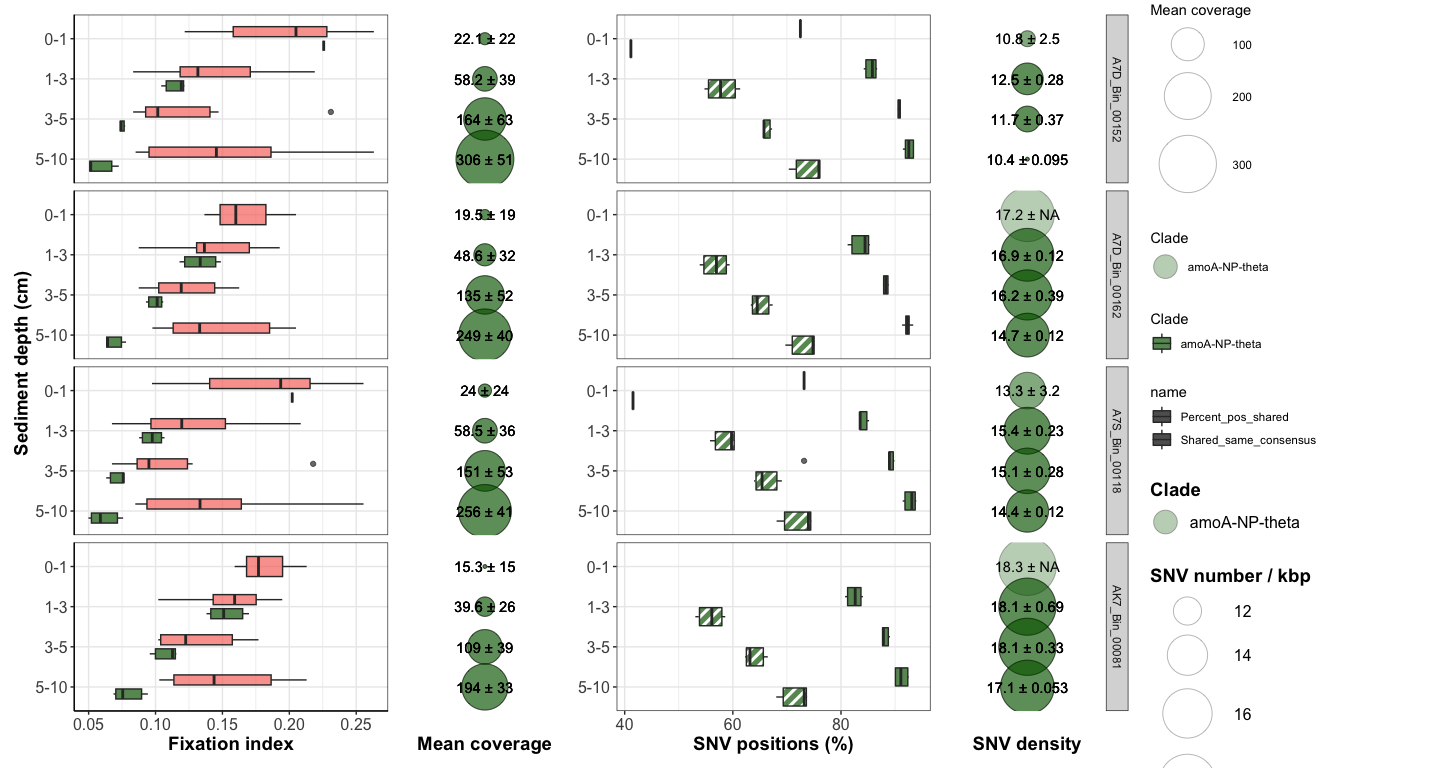
#dev.off()
# correlation of FST distance with shared SNVs ?
correlation <- right_join(FST_A7_long_full, df_shared_SNVs_long_full, by = c("Sample_1" = "Sample_ID_1", "Sample_2" = "Sample_ID_2", "Sample1_horizon", "Sample2_horizon", "Sample1_core", "Sample2_core", "Clade", "MAG_name"))
by(correlation, correlation$MAG_name, function(x) summary(lm(x$FST ~ x$Percent_pos_shared)))
## correlation$MAG_name: A7D_Bin_00152
##
## Call:
## lm(formula = x$FST ~ x$Percent_pos_shared)
##
## Residuals:
## Min 1Q Median 3Q Max
## -0.017510 -0.009818 -0.004600 0.012866 0.022105
##
## Coefficients:
## Estimate Std. Error t value Pr(>|t|)
## (Intercept) 0.3987398 0.0187535 21.26 3.34e-14 ***
## x$Percent_pos_shared -0.0047428 0.0002913 -16.28 3.24e-12 ***
## ---
## Signif. codes: 0 '***' 0.001 '**' 0.01 '*' 0.05 '.' 0.1 ' ' 1
##
## Residual standard error: 0.01301 on 18 degrees of freedom
## (2 observations deleted due to missingness)
## Multiple R-squared: 0.9364, Adjusted R-squared: 0.9329
## F-statistic: 265.2 on 1 and 18 DF, p-value: 3.238e-12
##
## ------------------------------------------------------------
## correlation$MAG_name: A7D_Bin_00162
##
## Call:
## lm(formula = x$FST ~ x$Percent_pos_shared)
##
## Residuals:
## Min 1Q Median 3Q Max
## -0.004698 -0.001445 0.001166 0.001500 0.004415
##
## Coefficients:
## Estimate Std. Error t value Pr(>|t|)
## (Intercept) 0.3564073 0.0068163 52.29 <2e-16 ***
## x$Percent_pos_shared -0.0039352 0.0001042 -37.75 <2e-16 ***
## ---
## Signif. codes: 0 '***' 0.001 '**' 0.01 '*' 0.05 '.' 0.1 ' ' 1
##
## Residual standard error: 0.003121 on 16 degrees of freedom
## (2 observations deleted due to missingness)
## Multiple R-squared: 0.9889, Adjusted R-squared: 0.9882
## F-statistic: 1425 on 1 and 16 DF, p-value: < 2.2e-16
##
## ------------------------------------------------------------
## correlation$MAG_name: A7S_Bin_00118
##
## Call:
## lm(formula = x$FST ~ x$Percent_pos_shared)
##
## Residuals:
## Min 1Q Median 3Q Max
## -0.014514 -0.010691 -0.002688 0.008601 0.020275
##
## Coefficients:
## Estimate Std. Error t value Pr(>|t|)
## (Intercept) 0.3588396 0.0188765 19.01 2.31e-13 ***
## x$Percent_pos_shared -0.0042602 0.0002953 -14.43 2.47e-11 ***
## ---
## Signif. codes: 0 '***' 0.001 '**' 0.01 '*' 0.05 '.' 0.1 ' ' 1
##
## Residual standard error: 0.0122 on 18 degrees of freedom
## (2 observations deleted due to missingness)
## Multiple R-squared: 0.9204, Adjusted R-squared: 0.916
## F-statistic: 208.1 on 1 and 18 DF, p-value: 2.473e-11
##
## ------------------------------------------------------------
## correlation$MAG_name: AK7_Bin_00081
##
## Call:
## lm(formula = x$FST ~ x$Percent_pos_shared)
##
## Residuals:
## Min 1Q Median 3Q Max
## -0.0054974 -0.0039417 -0.0000252 0.0011887 0.0083712
##
## Coefficients:
## Estimate Std. Error t value Pr(>|t|)
## (Intercept) 0.4129669 0.0105735 39.06 < 2e-16 ***
## x$Percent_pos_shared -0.0046909 0.0001647 -28.49 3.87e-15 ***
## ---
## Signif. codes: 0 '***' 0.001 '**' 0.01 '*' 0.05 '.' 0.1 ' ' 1
##
## Residual standard error: 0.00475 on 16 degrees of freedom
## (2 observations deleted due to missingness)
## Multiple R-squared: 0.9807, Adjusted R-squared: 0.9795
## F-statistic: 811.4 on 1 and 16 DF, p-value: 3.872e-15
by(correlation, correlation$MAG_name, function(x) summary(lm(x$FST ~ x$Shared_same_consensus)))
## correlation$MAG_name: A7D_Bin_00152
##
## Call:
## lm(formula = x$FST ~ x$Shared_same_consensus)
##
## Residuals:
## Min 1Q Median 3Q Max
## -0.0172594 -0.0029287 0.0004199 0.0048242 0.0083414
##
## Coefficients:
## Estimate Std. Error t value Pr(>|t|)
## (Intercept) 0.8207011 0.0202997 40.43 <2e-16 ***
## x$Shared_same_consensus -0.0082309 0.0002304 -35.73 <2e-16 ***
## ---
## Signif. codes: 0 '***' 0.001 '**' 0.01 '*' 0.05 '.' 0.1 ' ' 1
##
## Residual standard error: 0.006086 on 18 degrees of freedom
## (2 observations deleted due to missingness)
## Multiple R-squared: 0.9861, Adjusted R-squared: 0.9853
## F-statistic: 1276 on 1 and 18 DF, p-value: < 2.2e-16
##
## ------------------------------------------------------------
## correlation$MAG_name: A7D_Bin_00162
##
## Call:
## lm(formula = x$FST ~ x$Shared_same_consensus)
##
## Residuals:
## Min 1Q Median 3Q Max
## -0.012597 -0.003033 -0.002084 0.005822 0.006634
##
## Coefficients:
## Estimate Std. Error t value Pr(>|t|)
## (Intercept) 0.7536046 0.0308114 24.46 4.21e-14 ***
## x$Shared_same_consensus -0.0074133 0.0003495 -21.21 3.85e-13 ***
## ---
## Signif. codes: 0 '***' 0.001 '**' 0.01 '*' 0.05 '.' 0.1 ' ' 1
##
## Residual standard error: 0.005489 on 16 degrees of freedom
## (2 observations deleted due to missingness)
## Multiple R-squared: 0.9657, Adjusted R-squared: 0.9635
## F-statistic: 450 on 1 and 16 DF, p-value: 3.855e-13
##
## ------------------------------------------------------------
## correlation$MAG_name: A7S_Bin_00118
##
## Call:
## lm(formula = x$FST ~ x$Shared_same_consensus)
##
## Residuals:
## Min 1Q Median 3Q Max
## -0.080451 -0.006761 -0.000640 0.003732 0.045372
##
## Coefficients:
## Estimate Std. Error t value Pr(>|t|)
## (Intercept) 0.5303752 0.0739940 7.168 1.13e-06 ***
## x$Shared_same_consensus -0.0051054 0.0008542 -5.977 1.18e-05 ***
## ---
## Signif. codes: 0 '***' 0.001 '**' 0.01 '*' 0.05 '.' 0.1 ' ' 1
##
## Residual standard error: 0.02502 on 18 degrees of freedom
## (2 observations deleted due to missingness)
## Multiple R-squared: 0.6649, Adjusted R-squared: 0.6463
## F-statistic: 35.72 on 1 and 18 DF, p-value: 1.182e-05
##
## ------------------------------------------------------------
## correlation$MAG_name: AK7_Bin_00081
##
## Call:
## lm(formula = x$FST ~ x$Shared_same_consensus)
##
## Residuals:
## Min 1Q Median 3Q Max
## -0.0132476 -0.0025399 0.0002086 0.0039397 0.0050378
##
## Coefficients:
## Estimate Std. Error t value Pr(>|t|)
## (Intercept) 0.8517157 0.0248835 34.23 < 2e-16 ***
## x$Shared_same_consensus -0.0084580 0.0002848 -29.70 2.01e-15 ***
## ---
## Signif. codes: 0 '***' 0.001 '**' 0.01 '*' 0.05 '.' 0.1 ' ' 1
##
## Residual standard error: 0.00456 on 16 degrees of freedom
## (2 observations deleted due to missingness)
## Multiple R-squared: 0.9822, Adjusted R-squared: 0.9811
## F-statistic: 881.9 on 1 and 16 DF, p-value: 2.013e-15