ennoblement_16S
Electroactive bacteria associated with stainless steel ennoblement in seawater
This page contain a reproducible workflow for our paper on “Electroactive bacteria associated with stainless steel ennoblement in seawater”.
Table of content
- PART 1: From Raw sequencing data to the OTU table
- PART 2: Diversity, biomarkers and OTUs distribution
- PART 3: OCP and polarization curves
For the best reproducibility, the workflow can be used by setting you working directory in a $WD variable as follow
export WD="/path/to/your/working/directory/"
Raw data files can be accessed here and the fastq files are stored in the $WD/preprocess directory
PART 1: From Raw sequencing data to the OTU table
Quality filtering and paired end merging
The quality filtering and the paired end merging were performed with the Illumina-Utils python scripts written by Meren
Config file generation
cd $WD/preprocess/

# Create the first required file : qual-config.txt
ls *.fastq | \
awk 'BEGIN{FS="_R"}{print $1}' | \
uniq | \
awk 'BEGIN{print "sample\tr1\tr2"}
     {print $0 "\t" $0 "_R1.fastq\t" $0"_R2.fastq"}' > qual-config.txt

# Create the second required file : merge-config.txt
ls *.fastq | \
awk 'BEGIN{FS="_R"}{print $1}' | \
uniq | \
awk 'BEGIN{print "sample\tr1\tr2"}
     {print $0 "\t" $0 "-QUALITY_PASSED_R1.fastq\t" $0"-QUALITY_PASSED_R2.fastq"}' > merge-config.txt
Quality filtering
cd $WD/preprocess/

module load Illumina_Utils

iu-gen-configs qual-config.txt

# Loop for quality filtering
for i in *.ini
do
  iu-filter-quality-minoche $i
done
Paired end merging
cd $WD/preprocess/

# Generate .ini files with barcode (.....) and primer associated for both R1 and R2.
# Exact match will be kept, and barcode + primers will be trimmed during filtering.
iu-gen-configs merge-config.txt \
               --r1-prefix ^.....CCAGCAGC[C,T]GCGGTAA. \
               --r2-prefix CCGTC[A,T]ATT[C,T].TTT[A,G]A.T

# Loop for merging
for i in *.ini
do
  iu-merge-pairs $i
done
Dereplication
First af all, merged sequences are renamed and moved to fasta_dir
mkdir $WD/fasta_dir

# Copy merged fasta and change names
for i in `ls $WD/preprocess/ | grep MERGED | sed 's/\(^.*\)_MERGED/\1/'`
do
  cp $WD/preprocess/$i"_MERGED" $WD/fasta_dir/$i".fasta"
done
Dereplication and contingency table
module load Vsearch-2.3.4
mkdir $WD/swarm/
mkdir $WD/swarm/dereplicate

# Make sure all seq are lower case
for i in $WD/fasta_dir/*.fasta
do
  awk '{if(!/>/){print tolower($0)}else{print $0}}' $i > $i.temp | mv $i.temp $i
done


# For each fasta name in the fasta_dir, it dereplicates and rename seqs deflines
# If you wich to use the shell cammands provided by Fred Mahe, make sure DNA seqs are all upper (or lower) case.
for i in `ls $WD/fasta_dir/ | grep .fasta | sed 's/\(^.*\).fasta/\1/'`
do
  vsearch --derep_fulllength $WD/fasta_dir/$i.fasta \
          --sizeout \
          --relabel_sha1 \
          --fasta_width 0 \
          --output $WD/swarm/dereplicate/$i.derep.fasta
done


# Counting is in format: >Seq;size=#;
# But it need to be: >Seq_#
# To change it :
sed -i 's/size=/_/' $WD/swarm/dereplicate/*.derep.fasta
sed -i 's/;//g' $WD/swarm/dereplicate/*.derep.fasta

# Create a contingency table for unique seqs
# Thanks to Frederic Mahe https://github.com/torognes/swarm/wiki/Working-with-several-samples)
awk 'BEGIN {FS = "[>_]"}
           # Parse the sample files
           /^>/ {contingency[$2][FILENAME] = $3
           amplicons[$2] += $3
           if (FNR == 1) {
               samples[++i] = FILENAME
           }
          }
    END {# Create table header
          printf "amplicon"
          s = length(samples)
          for (i = 1; i <= s; i++) {
              printf "\t%s", samples[i]
          }
          printf "\t%s\n", "total"

          # Sort amplicons by decreasing total abundance (use a coprocess)
          command = "LC_ALL=C sort -k1,1nr -k2,2d"
          for (amplicon in amplicons) {
               printf "%d\t%s\n", amplicons[amplicon], amplicon |& command
          }
          close(command, "to")
          FS = "\t"
          while ((command |& getline) > 0) {
              amplicons_sorted[++j] = $2
          }
          close(command)

          # Print the amplicon occurrences in the different samples
          n = length(amplicons_sorted)
          for (i = 1; i <= n; i++) {
               amplicon = amplicons_sorted[i]
               printf "%s", amplicon
               for (j = 1; j <= s; j++) {
                   printf "\t%d", contingency[amplicon][samples[j]]
               }
               printf "\t%d\n", amplicons[amplicon]
          }}' $WD/swarm/dereplicate/*derep.fasta > $WD/swarm/amplicon_contingency_table.csv
Dereplication at the study level
export LC_ALL=C
cat $WD/swarm/dereplicate/*derep.fasta | \
awk 'BEGIN {RS = ">" ; FS = "[_\n]"}
     {if (NR != 1) {abundances[$1] += $2 ; sequences[$1] = $3}}
     END {for (amplicon in sequences) {
         print ">" amplicon "_" abundances[amplicon] "_" sequences[amplicon]}}' | \
sort --temporary-directory=$(pwd) -t "_" -k2,2nr -k1.2,1d | \
sed -e 's/\_/\n/2' > $WD/swarm/dereplicate/Temperature_effect.fasta
Swarm
module load Swarm-2.2.2

swarm -d 1 \
      -f \
      -t 8 \
      -s $WD/swarm/Temperature_effect.stat \
      -w $WD/swarm/OTUs_rep.fasta \
      -o $WD/swarm/Temperature_effect.swarm \
      -l $WD/swarm/Temperature_effect.log \
      $WD/swarm/dereplicate/Temperature_effect.fasta
OTU table
STATS="$WD/swarm/Temperature_effect.stat"
SWARMS="$WD/swarm/Temperature_effect.swarm"
AMPLICON_TABLE="$WD/swarm/amplicon_contingency_table.csv"
OTU_TABLE="$WD/swarm/OTU_contingency_table.csv"

# Header
echo -e "OTU\t$(head -n 1 "${AMPLICON_TABLE}")" > "${OTU_TABLE}"

# Compute "per sample abundance" for each OTU
awk -v SWARM="${SWARMS}" \
    -v TABLE="${AMPLICON_TABLE}" \
    'BEGIN {FS = " "
            while ((getline < SWARM) > 0) {
                swarms[$1] = $0
            }
            FS = "\t"
            while ((getline < TABLE) > 0) {
                table[$1] = $0
            }
           }

     {# Parse the stat file (OTUs sorted by decreasing abundance)
      seed = $3 "_" $4
      n = split(swarms[seed], OTU, "[ _]")
      for (i = 1; i < n; i = i + 2) {
          s = split(table[OTU[i]], abundances, "\t")
          for (j = 1; j < s; j++) {
              samples[j] += abundances[j+1]
          }
      }
      printf "%s\t%s", NR, $3
      for (j = 1; j < s; j++) {
          printf "\t%s", samples[j]
      }
     printf "\n"
     delete samples
     }' "${STATS}" >> "${OTU_TABLE}"
Chimera detection and removal
# Change size format from Swarm to Vsearch
sed -i 's/_/;size=/' $WD/swarm/OTUs_rep.fasta
sed -i 's/^>.*/&;/' $WD/swarm/OTUs_rep.fasta

vsearch --alignwidth 0 \
        --uchime_denovo $WD/swarm/OTUs_rep.fasta \
        --uchimeout $WD/swarm/Temperature_effect.uchimeout.txt

# Keep only the OTUs flagged as non-chimera
awk 'BEGIN{FS="\t"}{if ($18=="N") print $2}' $WD/swarm/Temperature_effect.uchimeout.txt > $WD/swarm/Temperature_effect.good_list.txt

# Remove the count number
sed -i 's/;size=.*;//g' $WD/swarm/Temperature_effect.good_list.txt

# Keep only non-chimera OTUs in the representative fasta
# Change ";size=" to "_"
sed -i 's/;size=/_/' $WD/swarm/OTUs_rep.fasta
sed -i 's/;//' $WD/swarm/OTUs_rep.fasta

awk 'NR==FNR{a[">"$0];next}BEGIN{FS="_"}{if ($1 in a){print $0; nr[NR+1]; next}}; NR in nr' $WD/swarm/Temperature_effect.good_list.txt OTUs_rep.fasta > $WD/swarm/OTUs_rep_chimera_free.fasta
Taxonomic Assignment
mkdir $WD/swarm/taxonomy
mkdir $WD/swarm/taxonomy/silva

# You need the Silva reference database. It was download in arb format and only
# the V4V5 region was kept to perform a quicker assignment
# A fasta and a taxonomic file are required for Mothur (https://mothur.org/wiki/Silva_reference_files)
cp /your/silva/Silva132_NR99_V4V5.fasta $WD/swarm/taxonomy/silva/
cp /your/silva/Silva132_NR99_V4V5.tax $WD/swarm/taxonomy/silva/

module load Mothur
cd $WD/swarm/taxonomy/
mothur "#classify.seqs(fasta=$WD/swarm/OTUs_rep_chimera_free.fasta, \
                       template=$WD/swarm/taxonomy/silva/Silva132_NR99_V4V5.fasta, \
                       taxonomy=$WD/swarm/taxonomy/silva/Silva132_NR99_V4V5.tax, \
                       processors=16)"
Complete OTU table
cp $WD/swarm/taxonomy/OTUs_rep_chimera_free.Silva132_NR99_V4V5.wang.taxonomy $WD/swarm/
sed -i 's/_/\t/' $WD/swarm/OTUs_rep_chimera_free.Silva132_NR99_V4V5.wang.taxonomy

# Add the taxonomy at the end of the otu table
awk 'NR==FNR{a[$1]=$3;next}{if ($1=="OTU"){print $0 "\ttaxonomy"}}{if ($2 in a){print $0 "\t" a[$2]; next}}; NR in nr' $WD/swarm/OTUs_rep_chimera_free.Silva132_NR99_V4V5.wang.taxonomy $WD/swarm/OTU_contingency_table.csv > $WD/swarm/Temperature_effect.complete_swarm_OTU_table.132.txt
PART 2: Diversity, biomarkers and OTUs distribution
Here are the required R pakages:
library("metagenomeSeq")
library("ggplot2")
library("reshape2")
library("vegan")
library("scales")
library("matrixStats")
library("data.table")
library("plyr")
Import and prepare the data
Import data and create the metadata table
Now we have an OTU table with an additional taxonomical assignment column.
full_df <- read.table("Temperature_effect.complete_swarm_OTU_table.132.txt", header = T, sep = "\t")
metadata <- data.frame(
  Sample_name = c(
    "X1B.derep.fasta", "X2B.derep.fasta",
    "X3B.derep.fasta", "X4B.derep.fasta",
    "X5B.derep.fasta", "X6B.derep.fasta",
    "X7B.derep.fasta", "X8B.derep.fasta",
    "X9B.derep.fasta", "X10B.derep.fasta",
    "X11B.derep.fasta", "X12B.derep.fasta",
    "X13B.derep.fasta", "X14B.derep.fasta",
    "X15B.derep.fasta", "X1C.derep.fasta",
    "X2C.derep.fasta", "X3C.derep.fasta",
    "X4C.derep.fasta", "X5C.derep.fasta",
    "X6C.derep.fasta", "X7C.derep.fasta",
    "X8C.derep.fasta", "X9C.derep.fasta",
    "X10C.derep.fasta", "X11C.derep.fasta",
    "X12C.derep.fasta", "X13C.derep.fasta",
    "X14C.derep.fasta", "X15C.derep.fasta",
    "S1_26mars15.derep.fasta",
    "S2_26mars15.derep.fasta",
    "S3_26mars15.derep.fasta",
    "S1_2mars15.derep.fasta",
    "S2_2mars15.derep.fasta",
    "S3_2mars15.derep.fasta"
  ),
  Group = c(
    "33°C", "33°C", "33°C", "33°C", "33°C", "30°C_1", "30°C_1",
    "30°C_1", "30°C_1", "30°C_1", "36°C", "36°C", "36°C", "36°C",
    "36°C", "40°C", "40°C", "40°C", "40°C", "40°C", "30°C_2",
    "30°C_2", "30°C_2", "30°C_2", "30°C_2", "38°C", "38°C",
    "38°C", "38°C", "38°C", "SW_23-02-15",
    "SW_23-02-15", "SW_23-02-15",
    "SW_02-02-15", "SW_02-02-15",
    "SW_02-02-15"
  ),
  ennobl = c(
    rep("ennoblement", 15),
    rep("non-ennoblement", 5),
    rep("ennoblement", 10),
    rep("non-ennoblement", 6)
  )
)
Remove unwanted OTUs from the dataset
We targeted Bacteria but some OTUs were identified as Chloroplast, Mitochondria, Archaea or Eukaryota. The remaining number of OTUs is in comments
full_df <- full_df[grep("Chloroplast", full_df$taxonomy, invert = T), ] # 69 234 OTUs
full_df <- full_df[grep("Mitochondria", full_df$taxonomy, invert = T), ] # 67 308 OTUs
full_df <- full_df[grep("Archaea", full_df$taxonomy, invert = T), ] # 67 180  OTUs
full_df <- full_df[grep("Eukaryota", full_df$taxonomy, invert = T), ] # 66 892 OTUs
OTU table format
Remove the taxonomic column and rename the rawname
samples <- as.character(metadata[, "Sample_name"])
all_df <- full_df[, samples]
row.names(all_df) <- full_df$amplicon
Count normalisation
The OTUs abundance were normalized with MetagenomeSeq
all_MR <- newMRexperiment(all_df)
all_MR_nor <- cumNorm(all_MR)
all_df_nor <- MRcounts(all_MR_nor, norm = T)
Create the taxonomic table
The taxonomy from the OTUs table is used to produce a complete taxonomic table.
It includes :
- Removal of the poor taxonomic assignment (under 80)
- Splitting of the taxonomy into the domain, phylum, etc
- Remove unclassified and uncultured
- Create a “short name” with the best taxonomic rank
- Make the assignment unique by adding the OTU number
full_taxonomy <- full_df[, c("amplicon", "taxonomy")]

# Replace poor taxonomic assignment (under 80) by 'unclassified'
full_taxonomy$taxonomy_80 <- apply(gsub(
  ".*\\(([1-7][0-9]|[0-9])\\)", "unclassified",
  strsplit2(as.character(full_taxonomy$taxonomy), ";")
),
1, paste,
collapse = ";"
)

# Split the taxonomy into domain, phylum, class, order, family, genus, species
full_taxonomy <- cbind(full_taxonomy, colsplit(full_taxonomy$taxonomy_80, "\\;",
  names = c(
    "domain", "phylum", "class", "order",
    "family", "genus", "species", "unclassified_col"
  )
))

# Remove 'unclassified'
full_taxonomy$taxonomy_80 <- gsub("unclassified;?", "", full_taxonomy$taxonomy_80)

# Remove 'uncultured'
full_taxonomy$taxonomy_80 <- gsub("uncultured.*", "", full_taxonomy$taxonomy_80)

# Retain only the last available taxonomic name starting from Species down to Domain
full_taxonomy$taxonomy_short <- sapply(
  strsplit(as.character(full_taxonomy$taxonomy_80), ";"),
  function(x) tail(x, n = 1)
)

# Make it unique by adding the OTU number
full_taxonomy$taxonomy_short <- paste0(
  full_taxonomy$taxonomy_short, " OTU",
  1:length(full_taxonomy$taxonomy_short)
)

# Make taxonomy unique
full_taxonomy$taxonomy_unique <- paste0(
  full_taxonomy$taxonomy_80,
  1:length(full_taxonomy$taxonomy_80)
)
Create color lists
# Colors for all samples
all_colors <- as.data.frame(matrix(c(
  "#1e972e", "#1d9e53", "#1cabaa", "#e7ce3e",
  "#d43c12", "#a30ca3", "#1c65ab", "#1c65ab",
  "30°C_1", "30°C_2", "33°C", "36°C", "38°C", "40°C",
  "SW_23-02-15", "SW_02-02-15"
), ncol = 2))

# Colors only for the temperature experiment
temp_colors <- as.data.frame(matrix(c(
  "#1e972e", "#1d9e53", "#1cabaa", "#e7ce3e",
  "#d43c12", "#a30ca3", "30°C_1", "30°C_2", "33°C",
  "36°C", "38°C", "40°C"
), ncol = 2))
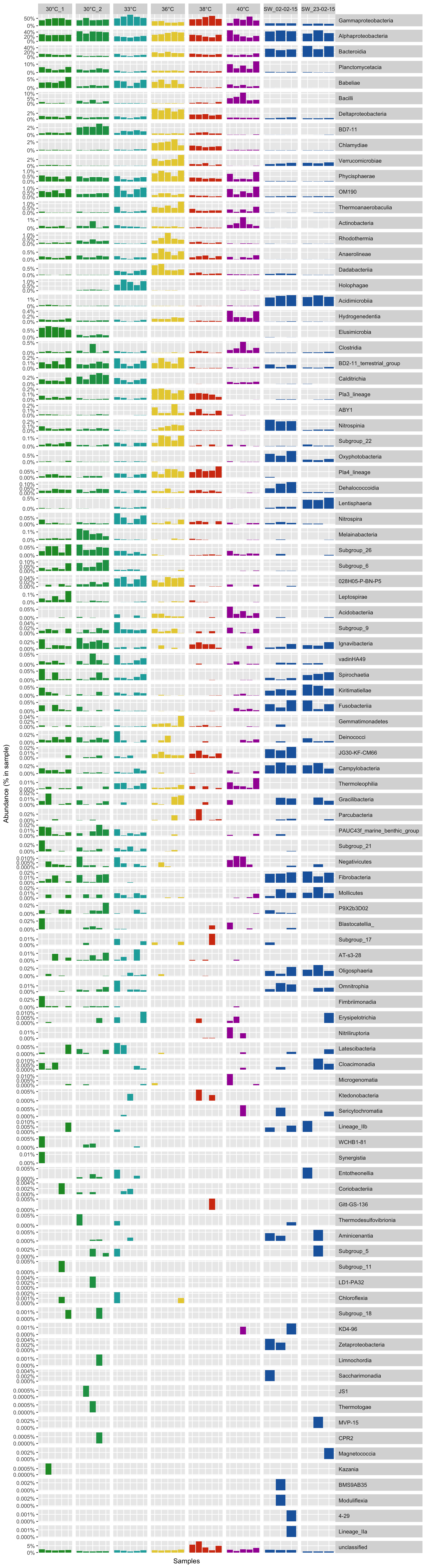
Overview of bacterial comunity
A the class level
# Get the Class per OTUs
class_level <- full_taxonomy[match(row.names(all_df_nor), full_taxonomy$amplicon), "class"]
class_level <- gsub("\\(.*", "", class_level)  # remove brackets -
class_level_df <- cbind(as.data.frame(all_df_nor), class_level)
class_level_df <- class_level_df[order(class_level_df$class_level),]

# sum sample abundance by Class
class_level_df <- aggregate(class_level_df[, 1:36], list(class_level_df$class_level), FUN = sum)
row.names(class_level_df) <- class_level_df$Group.1
class_level_df$Group.1 <- NULL
# order by max abunance
class_level_df <- class_level_df[order(rowSums(class_level_df), decreasing = T),]
class_level_df <- rbind(class_level_df[!row.names(class_level_df) == "unclassified", ], class_level_df[row.names(class_level_df) == "unclassified", ])
Prepare the data for the bar plot
# Transform the abundance in percentage
class_level_df <- t(t(class_level_df) / colSums(class_level_df))

# Melt the table and add metadata
class_level_dfm <- melt(t(class_level_df), varnames = c("sample", "otu"), value.name = "abundance")
class_level_dfm$group <- metadata[match(class_level_dfm$sample, metadata$Sample_name), "Group"]
class_level_dfm$taxa <- class_level_dfm$otu
Barplot function
P <- function(df, colors_list) {
  p <- ggplot(df, aes(sample, abundance, fill = group))
  p <- p + geom_bar(stat = "identity", position = "stack")
  p <- p + facet_grid(taxa ~ group, scales = "free")
  p <- p + scale_fill_manual(limits = as.vector(colors_list[[2]]), values = as.vector(colors_list[[1]]))
  p <- p + theme(
    legend.position = "", axis.ticks.x = element_blank(),
    strip.text.y = element_text(angle = 0, hjust = 0),
    panel.grid.minor = element_blank(), axis.text.x = element_blank()
  )
  p <- p + ylab("Abundance (% in sample)")
  p <- p + xlab("Samples")
  p <- p + scale_y_continuous(breaks = pretty_breaks(n = 2), labels = percent)
  print(p)
}
P(class_level_dfm, all_colors)
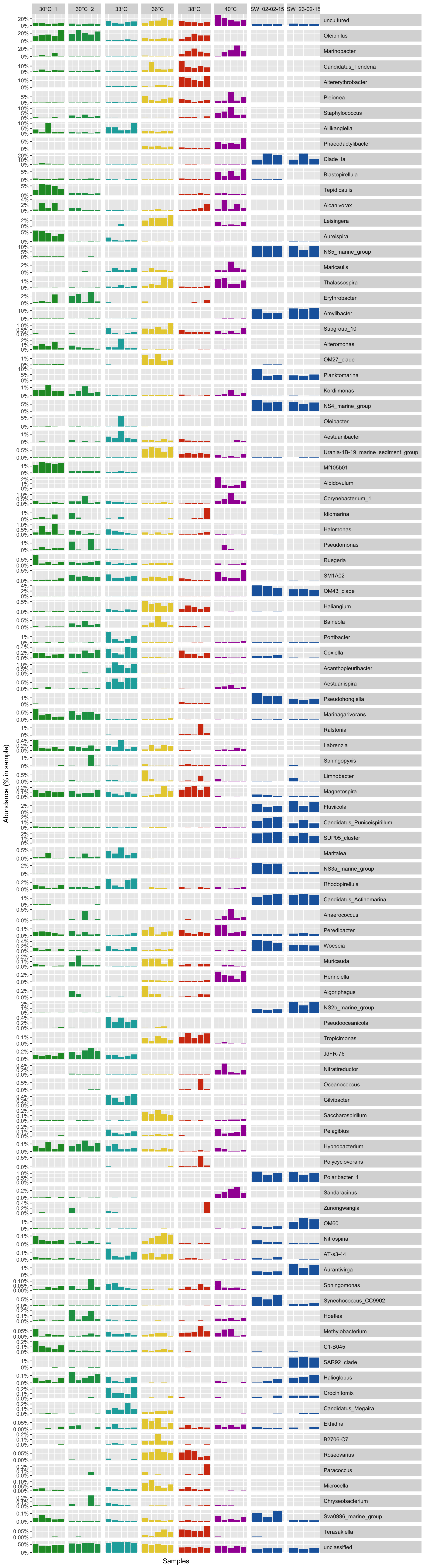
A the genus level
# Get the genus per OTUs
genus_level <- full_taxonomy[match(row.names(all_df_nor), full_taxonomy$amplicon), "genus"]
genus_level <- gsub("\\(.*", "", genus_level)  # remove brackets -
genus_level_df <- cbind(as.data.frame(all_df_nor), genus_level)
genus_level_df <- genus_level_df[order(genus_level_df$genus_level),]

# sum sample abundance by genus
genus_level_df <- aggregate(genus_level_df[, 1:36], list(genus_level_df$genus_level), FUN = sum)
row.names(genus_level_df) <- genus_level_df$Group.1
genus_level_df$Group.1 <- NULL
# order by max abunance
genus_level_df <- genus_level_df[order(rowSums(genus_level_df), decreasing = T),]
genus_level_df <- genus_level_df[1:100, ]
genus_level_df <- rbind(genus_level_df[!row.names(genus_level_df) == "unclassified", ], genus_level_df[row.names(genus_level_df) == "unclassified", ])
Prepare the data for the bar plot
# Transform the abundance in percentage
genus_level_df <- t(t(genus_level_df) / colSums(genus_level_df))

# Melt the table and add metadata
genus_level_dfm <- melt(t(genus_level_df), varnames = c("sample", "otu"), value.name = "abundance")
genus_level_dfm$group <- metadata[match(genus_level_dfm$sample, metadata$Sample_name), "Group"]
genus_level_dfm$taxa <- genus_level_dfm$otu
P(genus_level_dfm, all_colors)
Beta diversity
Split data with or without the seawater samples
# Transpose and select samples
all_tdf_nor <- t(all_df_nor)
temp_tdf_nor <- all_tdf_nor[1:30, ]
NMDS functions
Function for the ellipses
# Create the ellispe (http://stackoverflow.com/questions/13794419/plotting-ordiellipse-function-from-vegan-package-onto-nmds-plot-created-in-ggplo)
veganCovEllipse <- function(cov, center = c(0, 0), scale = 1, npoints = 100) {
  theta <- (0:npoints) * 2 * pi / npoints
  Circle <- cbind(cos(theta), sin(theta))
  t(center + scale * t(Circle %*% chol(cov)))
}
Ggplot function for the NMDS
P <- function(df, df_ell, colors_list, lab = "", title = "") {
  p <- ggplot(data = df, aes(x = NMDS1, y = NMDS2))
  p <- p + geom_polygon(
    data = df_ell, aes(x = NMDS1, y = NMDS2, fill = meta, color = meta),
    size = 0.5, linetype = 2, alpha = 0.2
  )
  p <- p + geom_point(size = 3, aes(fill = meta), col = "black", shape = 21, alpha = 1, stroke = 0.5)
  p <- p + scale_color_manual(
    limits = as.vector(colors_list[[2]]),
    values = as.vector(colors_list[[1]]),
    breaks = c("30°C_1", "33°C", "36°C", "38°C", "40°C", "SW_02-02-15"),
    labels = c("30°C", "33°C", "36°C", "38°C", "40°C", "Seawater")
  )
  p <- p + scale_fill_manual(
    limits = as.vector(colors_list[[2]]),
    values = as.vector(alpha(colors_list[[1]], 0.2)),
    breaks = c("30°C_1", "33°C", "36°C", "38°C", "40°C", "SW_02-02-15"),
    labels = c("30°C", "33°C", "36°C", "38°C", "40°C", "Seawater")
  )
  p <- p + labs(fill = lab, color = lab)
  p <- p + ggtitle(title)
  p <- p + theme(plot.title = element_text(face = "bold"))
  print(p)
}
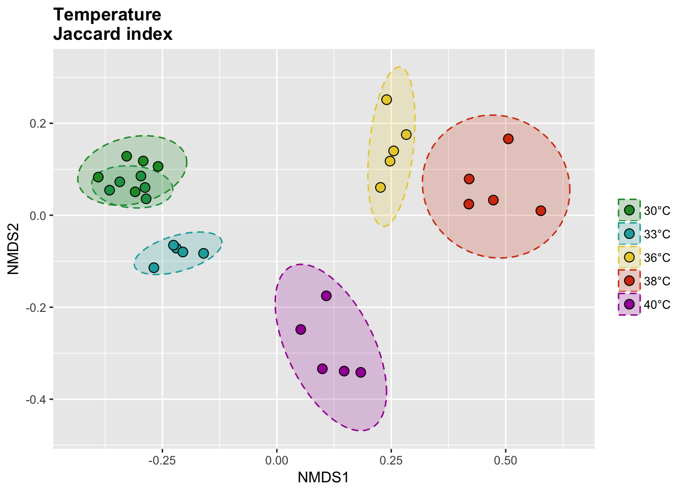
Temperature samples
Jaccard index
The binary Jaccard index compare sample bases on the presence/absence of OTUs, regardless of the relative abundance.
# Calcul distances
temp_jac_nor <- vegdist(temp_tdf_nor, method = "jaccard", binary = T)
temp_jac_nor_nmds <- metaMDS(temp_jac_nor)

# Extract NMDS scores and add the temperature value
temp_jac_nor_score <- as.data.frame(scores(temp_jac_nor_nmds))
temp_jac_nor_score$site <- rownames(temp_jac_nor_score)
temp_jac_nor_score$meta <- metadata$Group[match(temp_jac_nor_score$site, metadata$Sample_name)]
# Get data for ellipse
temp_jac_nor_ord <- ordiellipse(temp_jac_nor_nmds,
  group = as.character(metadata$Group[1:30]),
  kind = "sd", conf = 0.95, draw = c("none")
)

temp_jac_nor_ell <- data.frame()
for (g in unique(temp_jac_nor_score$meta)) {
  temp_jac_nor_ell <- rbind(
    temp_jac_nor_ell,
    cbind(as.data.frame(with(
      temp_jac_nor_score[temp_jac_nor_score$meta == g, ],
      veganCovEllipse(
        temp_jac_nor_ord[[g]]$cov,
        temp_jac_nor_ord[[g]]$center,
        temp_jac_nor_ord[[g]]$scale
      )
    )), meta = g)
  )
}
P(temp_jac_nor_score, temp_jac_nor_ell, temp_colors, "", title = "Temperature \nJaccard index")
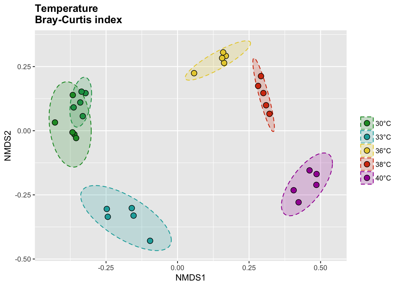
Bray-Curtis index
# Calcul distances
temp_bray_nor <- vegdist(temp_tdf_nor, method = "bray")
temp_bray_nor_nmds <- metaMDS(temp_bray_nor)

# Extract NMDS scores and add the temperature value
temp_bray_nor_score <- as.data.frame(scores(temp_bray_nor_nmds))
temp_bray_nor_score$site <- rownames(temp_bray_nor_score)
temp_bray_nor_score$meta <- metadata$Group[match(temp_bray_nor_score$site, metadata$Sample_name)]
# Get data for ellipse
temp_bray_nor_ord <- ordiellipse(temp_bray_nor_nmds,
  group = metadata$Group[1:30],
  kind = "sd", conf = 0.95, draw = c("none")
)

temp_bray_nor_ell <- data.frame()
for (g in unique(temp_bray_nor_score$meta)) {
  temp_bray_nor_ell <- rbind(
    temp_bray_nor_ell,
    cbind(as.data.frame(with(
      temp_bray_nor_score[temp_bray_nor_score$meta == g, ],
      veganCovEllipse(
        temp_bray_nor_ord[[g]]$cov,
        temp_bray_nor_ord[[g]]$center,
        temp_bray_nor_ord[[g]]$scale
      )
    )), meta = g)
  )
}
P(temp_bray_nor_score, temp_bray_nor_ell, temp_colors, "", title = "Temperature \nBray-Curtis index")
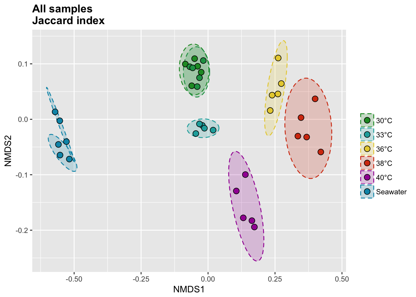
Temperature and seawater samples
Jaccard index
The binary Jaccard index compare sample bases on the presence/absence of OTUs, regardless of the relative abundance.
# Calcul distances
all_jac_nor <- vegdist(all_tdf_nor, method = "jaccard", binary = T)
all_jac_nor_nmds <- metaMDS(all_jac_nor)

# Extract NMDS scores and add the temperature value
all_jac_nor_score <- as.data.frame(scores(all_jac_nor_nmds))
all_jac_nor_score$site <- rownames(all_jac_nor_score)
all_jac_nor_score$meta <- metadata$Group[match(all_jac_nor_score$site, metadata$Sample_name)]
# Get data for ellipse
all_jac_nor_ord <- ordiellipse(all_jac_nor_nmds,
  group = as.character(metadata$Group),
  kind = "sd", conf = 0.95, draw = c("none")
)

all_jac_nor_ell <- data.frame()
for (g in unique(all_jac_nor_score$meta)) {
  all_jac_nor_ell <- rbind(
    all_jac_nor_ell,
    cbind(as.data.frame(with(
      all_jac_nor_score[all_jac_nor_score$meta == g, ],
      veganCovEllipse(
        all_jac_nor_ord[[g]]$cov,
        all_jac_nor_ord[[g]]$center,
        all_jac_nor_ord[[g]]$scale
      )
    )), meta = g)
  )
}
P(all_jac_nor_score, all_jac_nor_ell, all_colors, "", title = "All samples \nJaccard index")
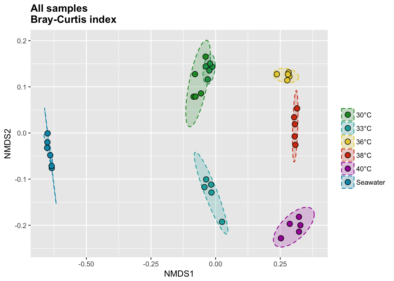
Bray-Curtis index
# Calcul distances
all_bray_nor <- vegdist(all_tdf_nor, method = "bray")
all_bray_nor_nmds <- metaMDS(all_bray_nor)

# Extract NMDS scores and add the temperature value
all_bray_nor_score <- as.data.frame(scores(all_bray_nor_nmds))
all_bray_nor_score$site <- rownames(all_bray_nor_score)
all_bray_nor_score$meta <- metadata$Group[match(all_bray_nor_score$site, metadata$Sample_name)]
# Get data for ellipse
all_bray_nor_ord <- ordiellipse(all_bray_nor_nmds,
  group = metadata$Group,
  kind = "sd", conf = 0.95, draw = c("none")
)

all_bray_nor_ell <- data.frame()
for (g in unique(all_bray_nor_score$meta)) {
  all_bray_nor_ell <- rbind(
    all_bray_nor_ell,
    cbind(as.data.frame(with(
      all_bray_nor_score[all_bray_nor_score$meta == g, ],
      veganCovEllipse(
        all_bray_nor_ord[[g]]$cov,
        all_bray_nor_ord[[g]]$center,
        all_bray_nor_ord[[g]]$scale
      )
    )), meta = g)
  )
}
P(all_bray_nor_score, all_bray_nor_ell, all_colors, "", title = "All samples \nBray-Curtis index")
Biomarker detection
Create and export the table for the LEfSe solftware
ennobl_lefse <- rbind(
  Class = as.character(metadata[match(colnames(all_df_nor), metadata$Sample_name), "ennobl"]),
  Sample = colnames(all_df_nor), all_df_nor
)
# Export the table
write.table(ennobl_lefse[, 1:30], "ennobl_lefse.txt", quote = F, sep = "\t", row.names = T, col.names = F)
Then in bash:
module load LEfSe

format_input.py ennobl_lefse.txt ennobl_lefse.in -c 1 -s -1 -u 2 -o 1000000
run_lefse.py -l 3 ennobl_lefse_only.in ennobl_lefse_only.out  # 47 features (LDA>3).
Import the result in R
ennobl_lefse_out <- read.table('ennobl_lefse_only.out', sep = '\t')
# Rename the columns
colnames(ennobl_lefse_out) <- c("features", "log_of_highest_class_average", "class", "LDA", "p_value")

# Remove NA line
ennobl_lefse_out <- ennobl_lefse_out[!is.na(ennobl_lefse_out$LDA), ]

# Order by decreasing LDA
ennobl_lefse_out <- ennobl_lefse_out[order(ennobl_lefse_out$LDA, decreasing = T), ]

# Remove unecessary "f_" at the begening of otu_ID
ennobl_lefse_out$features <- gsub("f_", "", ennobl_lefse_out$features)

# Add a taxa column
ennobl_lefse_out$taxonomy <- full_taxonomy[match(ennobl_lefse_out$features, full_taxonomy$amplicon), "taxonomy_short"]
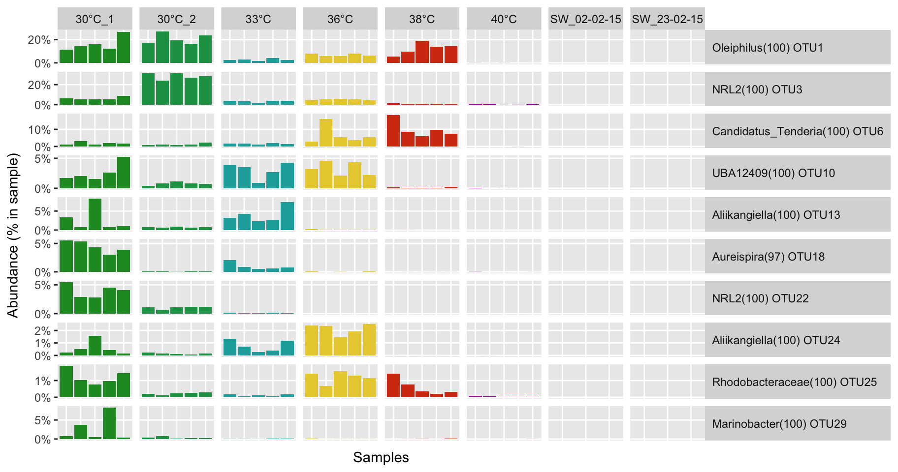
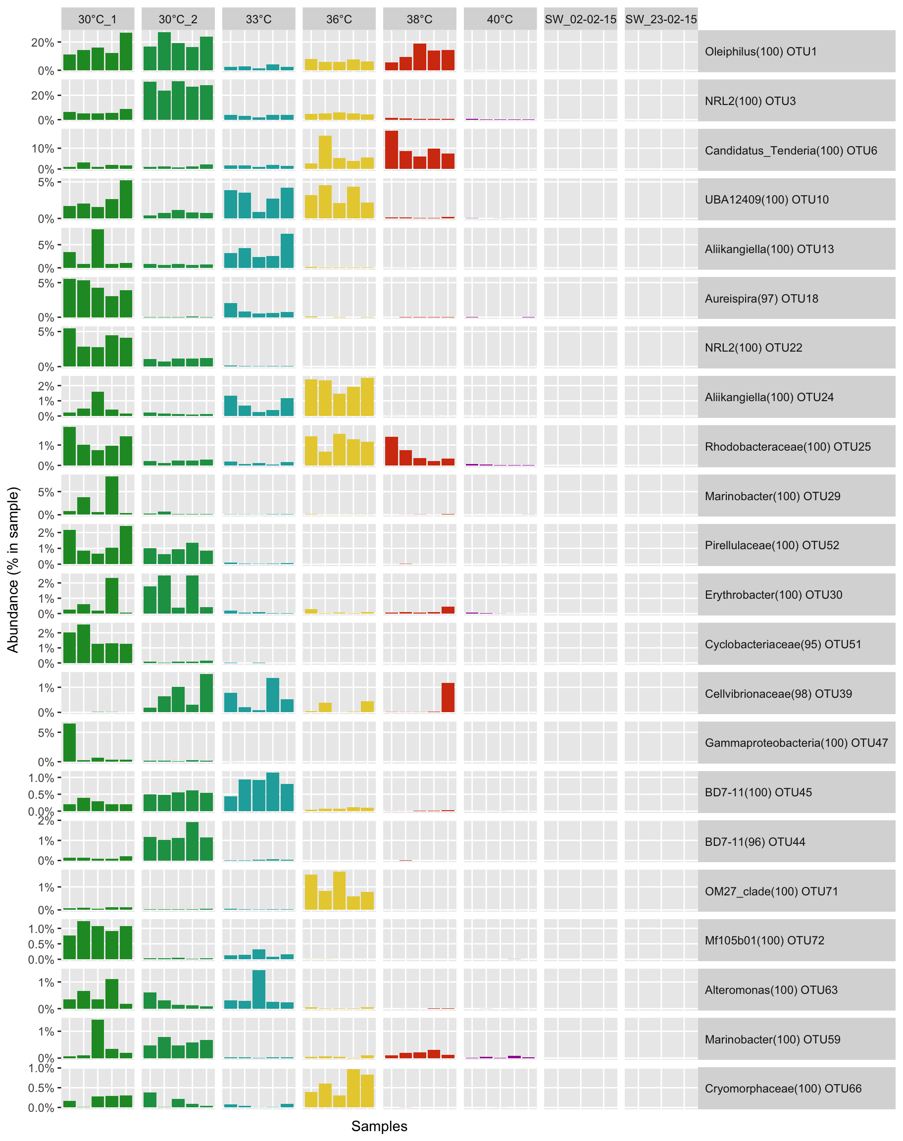
Prepare the data for the bar plot
# Select biomarker of the condition ennoblement and remove the non-ennoblement features
ennobl_only_lefse_out <- ennobl_lefse_out[ennobl_lefse_out$class == "ennoblement", "features"]

# Extract biomarker OTUs
ennobl_only_lefse_df <- all_df_nor[ennobl_only_lefse_out, ]

# Transform the abundance in percentage
ennobl_only_lefse_df <- t(t(ennobl_only_lefse_df) / colSums(all_df_nor))

# Select top 10
ennobl_only_lefse_top10_df <- ennobl_only_lefse_df[1:10, ]

# Melt the table and add metadata
ennobl_only_lefse_dfm <- melt(t(ennobl_only_lefse_df), varnames = c("sample", "otu"), value.name = "abundance")
ennobl_only_lefse_dfm$group <- metadata[match(ennobl_only_lefse_dfm$sample, metadata$Sample_name), "Group"]
ennobl_only_lefse_dfm$taxa <- factor(
  full_taxonomy[match(ennobl_only_lefse_dfm$otu, full_taxonomy$amplicon), "taxonomy_short"],
  levels = unique(full_taxonomy[match(ennobl_only_lefse_dfm$otu, full_taxonomy$amplicon), "taxonomy_short"])
)

# Melt the table and add metadata for the top 10
ennobl_only_lefse_top10_dfm <- melt(t(ennobl_only_lefse_top10_df), varnames = c("sample", "otu"), value.name = "abundance")
ennobl_only_lefse_top10_dfm$group <- metadata[match(ennobl_only_lefse_top10_dfm$sample, metadata$Sample_name), "Group"]
ennobl_only_lefse_top10_dfm$taxa <- factor(
  full_taxonomy[match(ennobl_only_lefse_top10_dfm$otu, full_taxonomy$amplicon), "taxonomy_short"],
  levels = unique(full_taxonomy[match(ennobl_only_lefse_top10_dfm$otu, full_taxonomy$amplicon), "taxonomy_short"])
)
Barplot function
P <- function(df, colors_list) {
  p <- ggplot(df, aes(sample, abundance, fill = group))
  p <- p + geom_bar(stat = "identity", position = "stack")
  p <- p + facet_grid(taxa ~ group, scales = "free")
  p <- p + scale_fill_manual(limits = as.vector(colors_list[[2]]), values = as.vector(colors_list[[1]]))
  p <- p + theme(
    legend.position = "", axis.ticks.x = element_blank(),
    strip.text.y = element_text(angle = 0, hjust = 0),
    panel.grid.minor = element_blank(), axis.text.x = element_blank()
  )
  p <- p + ylab("Abundance (% in sample)")
  p <- p + xlab("Samples")
  p <- p + scale_y_continuous(breaks = pretty_breaks(n = 2), labels = percent)
  print(p)
}
P(ennobl_only_lefse_top10_dfm, temp_colors)
P(ennobl_only_lefse_dfm, temp_colors)
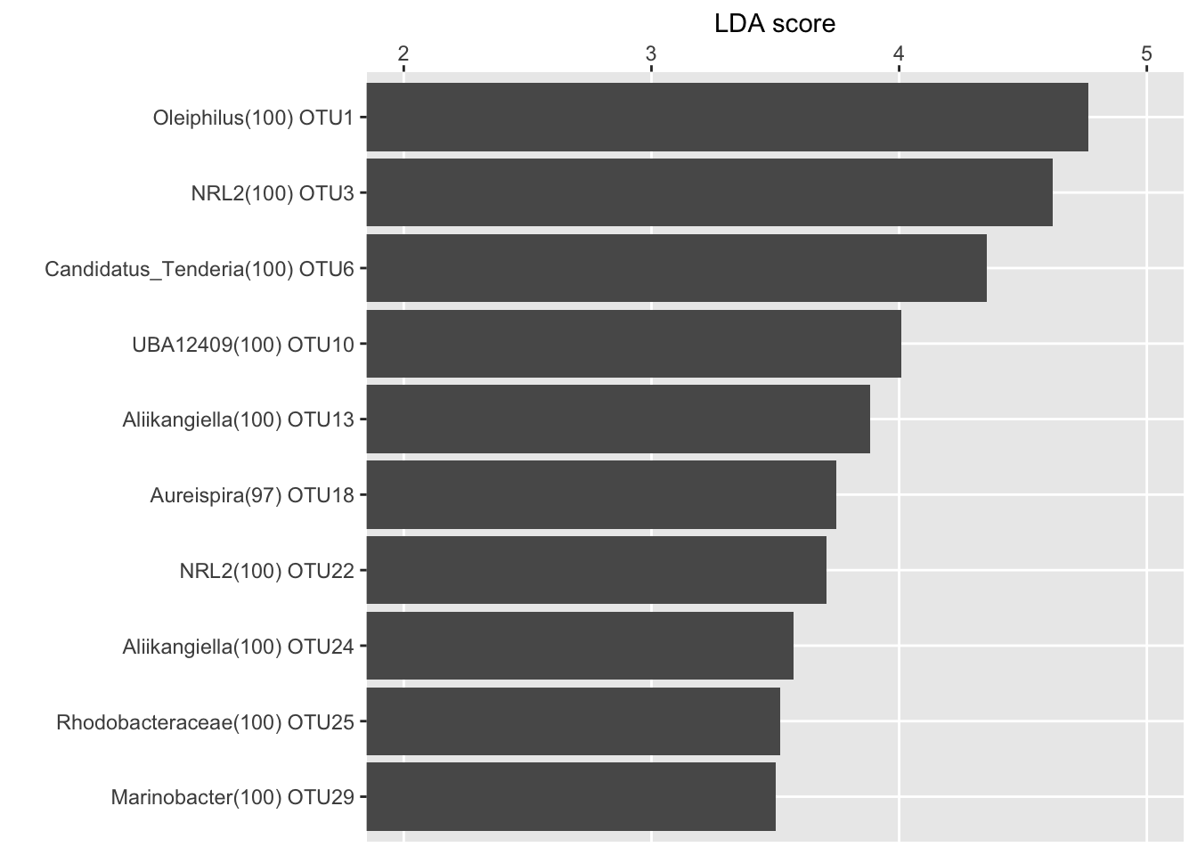
LDA score for the top 10 biomarkers
ennobl_only_lefse_lda <- ennobl_lefse_out[ennobl_lefse_out$class == "ennoblement", ]
ennobl_only_lefse_lda <- ennobl_only_lefse_lda[1:10, ]
ennobl_only_lefse_lda <- ennobl_only_lefse_lda[order(ennobl_only_lefse_lda$LDA, decreasing = F), ]
ennobl_only_lefse_lda$taxonomy <- factor(ennobl_only_lefse_lda$taxonomy,
  levels = ennobl_only_lefse_lda$taxonomy
)
LDA <- function(df) {
  p <- ggplot(df, aes(taxonomy, LDA))
  p <- p + geom_bar(stat = "identity", position = "stack")
  p <- p + theme(
    legend.position = "", panel.grid.minor = element_blank(),
    strip.text.x = element_text(angle = 0, hjust = 0)
  )
  p <- p + ylab("LDA score")
  p <- p + xlab("")
  p <- p + scale_y_continuous(position = "right")
  p <- p + coord_flip(ylim = c(2, 5))
  print(p)
}
LDA(ennobl_only_lefse_lda)
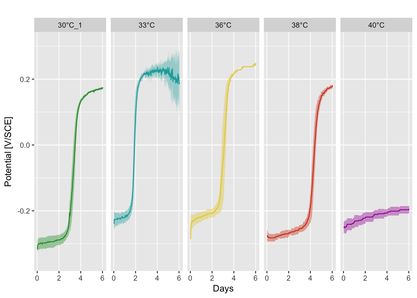
PART 3: OCP and polarization curves
Open circuit potential
Data were collected with four Embedded Personal Computer (EPC). A Ag/AgCl reference electrode was used for each conditions and calibrated with a Saturated Calomel Electrode (SCE)
EPC_1 <- read.table(file = "EPC_1.30&33_degree", header = T, sep = ";")
EPC_2 <- read.table(file = "EPC_2.30&36_degree", header = T, sep = ";")
EPC_3 <- read.table(file = "EPC_3.30&40_degree", header = T, sep = ";")
EPC_4 <- read.table(file = "EPC_4.30&38_degree", header = T, sep = ";")
# Ensure that all data are the same length
EPC_1 <- EPC_1[1:290, ]
EPC_2 <- EPC_2[1:290, ]
EPC_3 <- EPC_3[1:290, ]
EPC_4 <- EPC_4[1:290, ]

# Merge all data and remove the first column to avoid repeated $date
All_EPC <- data.frame(EPC_1, EPC_2[, -1], EPC_3[, -1], EPC_4[, -1])

# Reference electrode calibration (Ag/AgCl to SCE)
df <- data.frame(
  All_EPC[, c(2:6)] + 0.010,
  All_EPC[, c(7:11)] - 0.022,
  All_EPC[, c(12:16)] + 0.018,
  All_EPC[, c(17:21)] + 0.015,
  All_EPC[, c(22:26)] - 0.022,
  All_EPC[, c(27:31)] - 0.004
)

df <- as.matrix(df)
# Calcul the mean and 95% confidence interval per condition
df <- data.frame(
  mean_30 = rowMeans(df[, c(6:10, 21:25)]),
  positive_sd_30 = rowMeans(df[, c(6:10, 21:25)]) + (1.96 * rowSds(df[, c(6:10, 21:25)]) / sqrt(10)),
  negative_sd_30 = rowMeans(df[, c(6:10, 21:25)]) - (1.96 * rowSds(df[, c(6:10, 21:25)]) / sqrt(10)),
  mean_33 = rowMeans(df[, 1:5]),
  positive_sd_33 = rowMeans(df[, 1:5]) + (1.96 * rowSds(df[, 1:5]) / sqrt(5)),
  negative_sd_33 = rowMeans(df[, 1:5]) - (1.96 * rowSds(df[, 1:5]) / sqrt(5)),
  mean_36 = rowMeans(df[, 11:15]),
  positive_sd_36 = rowMeans(df[, 11:15]) + (1.96 * rowSds(df[, 11:15]) / sqrt(5)),
  negative_sd_36 = rowMeans(df[, 11:15]) - (1.96 * rowSds(df[, 11:15]) / sqrt(5)),
  mean_38 = rowMeans(df[, 26:30]),
  positive_sd_38 = rowMeans(df[, 26:30]) + (1.96 * rowSds(df[, 26:30]) / sqrt(5)),
  negative_sd_38 = rowMeans(df[, 26:30]) - (1.96 * rowSds(df[, 26:30]) / sqrt(5)),
  mean_40 = rowMeans(df[, 16:20]),
  positive_sd_40 = rowMeans(df[, 16:20]) + (1.96 * rowSds(df[, 16:20]) / sqrt(5)),
  negative_sd_40 = rowMeans(df[, 16:20]) - (1.96 * rowSds(df[, 16:20]) / sqrt(5)),
  Time_days = as.numeric(row.names(df)) / 48
)
# Melt the dataframe
df.mean <- melt(df[, c(1, 4, 7, 10, 13, 16)], id.vars = "Time_days")

# Remove the 2 extreme value from sample 33°C
df.mean <- df.mean[-c(432, 433), ]

# Melt confidence interval values
df.sd <- rbind(
  melt(setnames(df[, c(2, 16)], old = "positive_sd_30", new = "mean_30"), id.vars = "Time_days"),
  melt(setnames(df[rev(row.names(df)), c(3, 16)], old = "negative_sd_30", new = "mean_30"),
    id.vars = "Time_days"
  ),
  melt(setnames(df[, c(5, 16)], old = "positive_sd_33", new = "mean_33"), id.vars = "Time_days"),
  melt(setnames(df[rev(row.names(df)), c(6, 16)], old = "negative_sd_33", new = "mean_33"),
    id.vars = "Time_days"
  ),
  melt(setnames(df[, c(8, 16)], old = "positive_sd_36", new = "mean_36"), id.vars = "Time_days"),
  melt(setnames(df[rev(row.names(df)), c(9, 16)], old = "negative_sd_36", new = "mean_36"),
    id.vars = "Time_days"
  ),
  melt(setnames(df[, c(11, 16)], old = "positive_sd_38", new = "mean_38"), id.vars = "Time_days"),
  melt(setnames(df[rev(row.names(df)), c(12, 16)], old = "negative_sd_38", new = "mean_38"),
    id.vars = "Time_days"
  ),
  melt(setnames(df[, c(14, 16)], old = "positive_sd_40", new = "mean_40"), id.vars = "Time_days"),
  melt(setnames(df[rev(row.names(df)), c(15, 16)], old = "negative_sd_40", new = "mean_40"),
    id.vars = "Time_days"
  )
)

# Remove aberrant values at 33°C
df.sd <- df.sd[-c(722, 723, 1018, 1019), ]
Ggplot function
P <- function(df.mean, df.sd, colors_list) {
  p <- ggplot(df.mean, aes(x = Time_days, y = value, color = variable))
  p <- p + geom_polygon(data = df.sd, aes(x = Time_days, y = value, fill = variable, color = NA))
  p <- p + geom_line()
  p <- p + facet_grid(~variable)
  p <- p + scale_color_manual(
    limits = as.vector(colors_list[[2]]),
    values = as.vector(colors_list[[1]]),
    breaks = c("30°C_1", "33°C", "36°C", "38°C", "40°C", "SW_02-02-15"),
    labels = c("30°C", "33°C", "36°C", "38°C", "40°C", "Seawater")
  )
  p <- p + scale_fill_manual(
    limits = as.vector(colors_list[[2]]),
    values = alpha(as.vector(colors_list[[1]]), 0.4),
    breaks = c("30°C_1", "33°C", "36°C", "38°C", "40°C", "SW_02-02-15"),
    labels = c("30°C", "33°C", "36°C", "38°C", "40°C", "Seawater")
  )
  p <- p + scale_x_continuous(breaks = seq(0, 14, 2))
  p <- p + scale_y_continuous(limits = c(-0.35, 0.31))
  p <- p + labs(x = "Days", y = "Potential [V/SCE]", title = "")
  p <- p + theme(
    legend.position = "none", panel.grid.minor.x = element_blank(),
    panel.grid.major.x = element_line(color = "grey98")
  )
  print(p)
}
P(df.mean, df.sd, temp_colors)
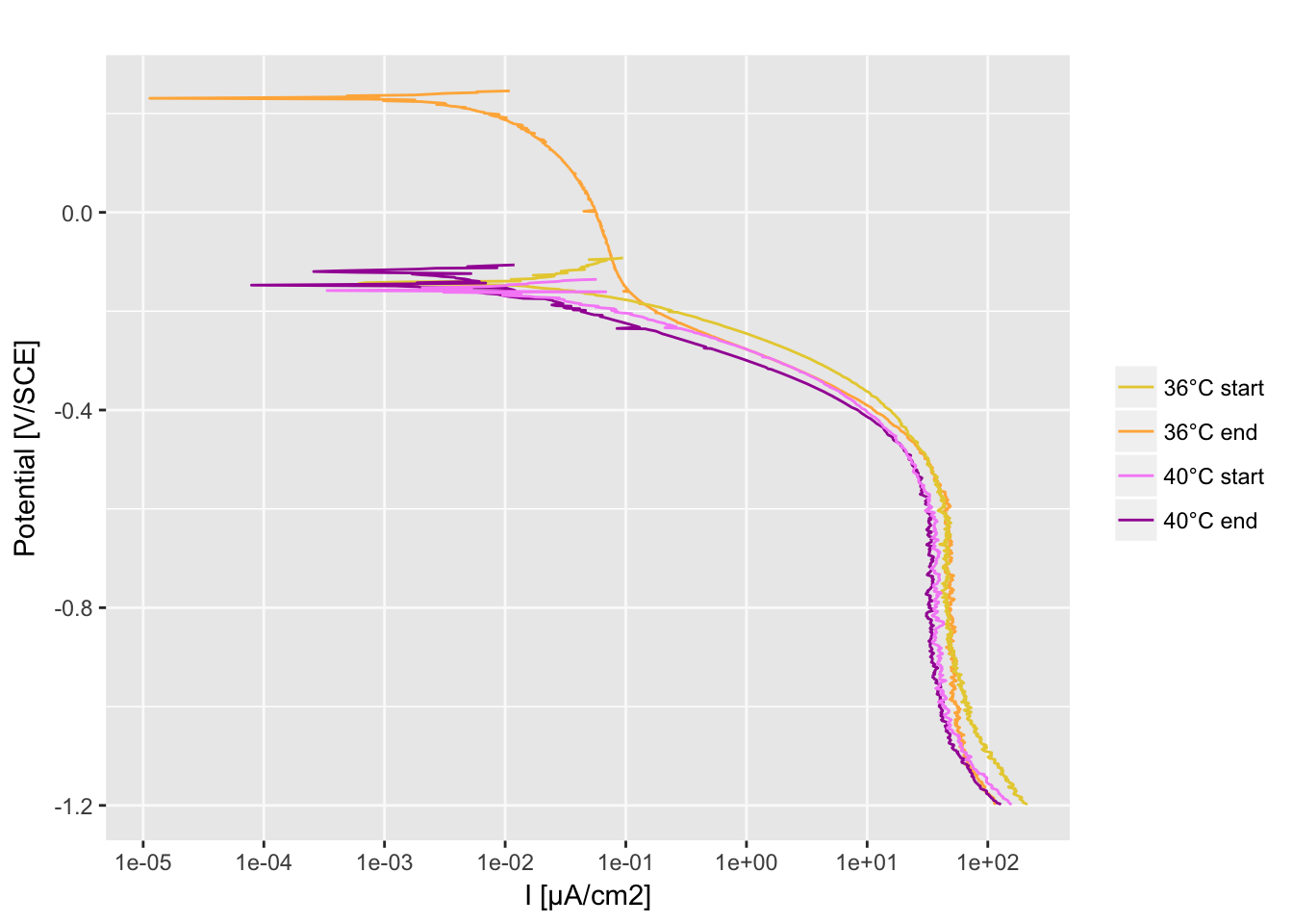
Cathodic polarization curves
Import the data
df_36deg_start <- read.table(file = "30°start_CATHODIC.txt", header = T, dec = ",")
df_36deg_end <- read.table(file = "36°end_CATHODIC.txt", header = T, dec = ",")
df_40deg_start <- read.table(file = "40°start_CATHODIC.txt", header = T, dec = ",")
df_40deg_end <- read.table(file = "40°end_CATHODIC.txt", header = T, dec = ",")
colors_list <- as.data.frame(matrix(c(
  "#ffb347",
  "#e7ce3e",
  "#a30ca3",
  "#f790f7",
  "36deg_end",
  "36deg_start",
  "40deg_end",
  "40deg_start"
), ncol = 2))

# Sample size to convert current to current density
len <- 10 # length (cm)
wid <- 1 # width (cm)
hei <- 5 # height (cm)
coupon_surface <- (2 * len * wid + 2 * len * hei + 2 * wid * hei) # coupon area (cm2)
A function to prepare the data:
- Remove Overload value
- Add sample name and metadata
- Convert the current to current density (µA/cm2)
data_prep <- function(data, ID = "", group = "") {
data <- data[data$Over == "...........", ]
data$sampleID <- ID
data$group <- group
data$Im <- abs(as.numeric(as.character(data$Im)))
data$Im <- data$Im / coupon_surface * 1e+06
data$Vf <- as.numeric(as.character(data$Vf))
return(data)
}
# Apply the function to the 4 conditions
df_36deg_start <- data_prep(df_36deg_start, "36deg_start", "36deg_start")
df_36deg_end <- data_prep(df_36deg_end, "36deg_end", "36deg_end")
df_40deg_start <- data_prep(df_40deg_start, "40deg_start", "40deg_start")
df_40deg_end <- data_prep(df_40deg_end, "40deg_end", "40deg_end")

df <- rbind(
  df_36deg_start,
  df_36deg_end,
  df_40deg_start,
  df_40deg_end
)
Ggplot function
P <- function(dfm, colors_list) {
  p <- ggplot(dfm[, ], aes(x = Im, y = Vf, group = sampleID, color = group))
  p <- p + geom_path()
  p <- p + scale_color_manual(
    limits = as.vector(colors_list[[2]]),
    values = as.vector(alpha(colors_list[[1]])),
    breaks = c("36deg_start", "36deg_end", "40deg_start", "40deg_end"),
    labels = c("36°C start", "36°C end", "40°C start", "40°C end")
  )
  p <- p + labs(x = "I [µA/cm2]", y = "Potential [V/SCE]", title = "")
  p <- p + scale_x_continuous(breaks = c(10^-5, 10^-4, 10^-3, 10^-2, 10^-1, 1, 10^+1, 10^+2), trans = "log10")
  p <- p + theme(
    panel.grid.major.x = element_line(color = "grey98"),
    panel.grid.major.y = element_line(color = "grey98"),
    panel.grid.minor.x = element_blank(), legend.title = element_blank()
  )
  print(p)
}
P(df, colors_list)